当前位置:网站首页>Data processing in detailed machine learning (II) -- Feature Normalization
Data processing in detailed machine learning (II) -- Feature Normalization
2022-06-13 02:36:00 【Infinite thoughts】

Abstract : In machine learning , Our data sets often have a variety of problems , If you don't preprocess the data , It is difficult to train and predict the model . This series of blog posts will introduce the problem of data preprocessing in machine learning , With U C I \color{#4285f4}{U}\color{#ea4335}{C}\color{#fbbc05}{I} UCI Take dataset as an example to introduce missing value processing in detail 、 Continuous feature discretization , Feature normalization and coding of discrete features , At the same time, the handling will be attached M a t l a b \color{#4285f4}{M}\color{#ea4335}{a}\color{#fbbc05}{t}\color{#4285f4}{l}\color{#34a853}{a}\color{#ea4335}{b} Matlab Program code , This blog first introduces feature normalization , The contents are as follows :
List of articles
Preface
In this blog post, I will focus on the topics that are often used in machine learning U C I \color{#4285f4}{U}\color{#ea4335}{C}\color{#fbbc05}{I} UCI Data set as an example . About U C I \color{#4285f4}{U}\color{#ea4335}{C}\color{#fbbc05}{I} UCI Introduction and collation of data sets , In my previous two blog posts :UCI Detailed explanation of data set and its data processing ( attach 148 Data sets and processing code )、UCI Data set collation ( Attached are the commonly used data sets of papers ) They all have a detailed introduction , Interested readers can click to learn about it .
It is said that ,“ one can't make bricks without straw ”. In machine learning , Data and characteristics are “ rice ”, The model and the algorithm are “ housewife ”. There's not enough data 、 Appropriate features , No matter how powerful the model structure is, it can't get satisfactory output . As an industry classic saying goes ,“Garbage in,garbage out”. For a machine learning problem , Data and characteristics often determine the upper limit of results , And the model 、 The selection and optimization of algorithms are gradually approaching this upper limit .
1. Feature normalization
Feature Engineering , seeing the name of a thing one thinks of its function , It is a series of engineering processing for the original data , Refine it into characteristics , As input for algorithms and models . essentially , Feature engineering is a process of representing and presenting data . In practice , Feature engineering is designed to remove impurities and redundancy from raw data , Design more efficient features to depict the relationship between the problem solved and the prediction model .
Both normalization and standardization can make features dimensionless , Normalization makes the data shrink to [0, 1] And make the weights of features the same , Changed the distribution of the original data ; Standardization makes the features of different measures comparable by scaling the different feature dimensions , At the same time, it does not change the distribution of the original data . The method of the next section is partly quoted from Zhuge Yue 、 Gourd baby's 《 Baimian machine learning 》 Introduction to the normalization of specific values .
Feature normalization method
In order to eliminate the dimensional impact between data features , We need to normalize the features , Make different indicators comparable . for example , Analyze the health effects of a person's height and weight , If you use rice (m) And kilogram (kg) As a unit , Then the height characteristics will be in 1.6~1.8m Within the numerical range of , The weight characteristics will be in 50~100kg Within the scope of , The results of the analysis will obviously tend to the weight characteristics with large numerical difference . Want to get more accurate results , We need to normalize the features (Normalization) Handle , Make each index in the same numerical magnitude , For analysis .
By normalizing the features of numerical type, all features can be unified into a roughly same numerical range . The most commonly used methods are as follows .
(1) Normalization of linear function (Min-Max Scaling): It's a linear transformation of raw data , Map the results to [0, 1] The scope of the , Realize the scaling of the original data . The normalization formula is as follows :
X n o r m = X − X m i n X m a x − X m i n (1.1) X_{norm}=\frac{X-X_{min}}{X_{max}-X_{min}}\tag{1.1} Xnorm=Xmax−XminX−Xmin(1.1)
among X X X For raw data , X m a x X_{max} Xmax、 X m i n X_{min} Xmin Maximum and minimum values of data .
(2) Zero mean normalization (Z-Score Normalization): It maps the raw data to a mean of 0、 The standard deviation is 1 The distribution of . say concretely , Assume that the mean value of the original feature is μ \mu μ、 The standard deviation is σ \sigma σ, So the normalization formula is defined as :
z = x − μ σ (1.2) z=\frac{x-\mu }{\sigma }\tag{1.2} z=σx−μ(1.2)
Why do we need to normalize numerical features ? We might as well use the example of random gradient descent to illustrate the importance of normalization . Suppose there are two numerical characteristics , x 1 x_{1} x1 The value range of is [0, 10], x 2 x_{2} x2 The value range of is [0, 3], So we can construct an objective function coincidence graph 1.1 (a) Isogram in . At the same learning rate , x 1 x_{1} x1 The update speed of will be greater than x 2 x_{2} x2, It takes more iterations to find the optimal solution . If you will x 1 x_{1} x1 and x 2 x_{2} x2 After normalization to the same numerical range , The contour map of the optimization target will become a graph 1.1 (b) Circle in , x 1 x_{1} x1 and x 2 x_{2} x2 The update speed of becomes more consistent , It is easy and faster to find the optimal solution through gradient descent .

in application , The model solved by gradient descent method usually needs normalization , Including linear regression 、 Logical regression 、 Support vector machine 、 Neural networks and other models . Of course , Data normalization is not everything , This method is not applicable to the decision tree model .
Matlab Code implementation
Here I will introduce you how to use code to realize . stay M a t l a b \color{#4285f4}{M}\color{#ea4335}{a}\color{#fbbc05}{t}\color{#4285f4}{l}\color{#34a853}{a}\color{#ea4335}{b} Matlab The two normalization methods mentioned above have their own processing functions , To avoid secondary development, we use its own functions , They are maximum and minimum mapping respectively :mapminmax( ) and z Value standardization :zscore( ). Here we introduce the following two functions respectively ,mapminmax( ) Function official documentation Introduce the following :
mapminmax
By mapping the minimum and maximum values of rows to [ -1 1] To handle the matrix
grammar
[Y,PS] = mapminmax(X,YMIN,YMAX)
[Y,PS] = mapminmax(X,FP)
Y = mapminmax(‘apply’,X,PS)
explain
[Y,PS] = mapminmax(X,YMIN,YMAX) By normalizing the minimum and maximum values of each row to [ YMIN,YMAX] To handle the matrix .
[Y,PS] = mapminmax(X,FP) Use structure as a parameter : FP.ymin,FP.ymax.
Y = mapminmax(‘apply’,X,PS) Given X And set up PS, return Y.——MATLAB Official documents
mapminmax( ) Functions are normalized by row , We can test by typing instructions on the command line , Because the data attributes in the dataset are by column, the matrix needs to be transposed during calculation , The test instructions and running results are as follows :
>> x1 = [1 2 4; 1 1 1; 3 2 2; 0 0 0]

x1 =

     1     2     4
     1     1     1
     3     2     2
     0     0     0

>> [y1,PS] = mapminmax(x1'); >> y1'

ans =

   -0.3333    1.0000    1.0000
   -0.3333         0   -0.5000
    1.0000    1.0000         0
   -1.0000   -1.0000   -1.0000
zscore( ) The documentation for the use of is as follows , This function normalizes each element by column to the mean value to 0, The standard deviation is 1 The distribution of , Please refer to zscore( ) Function official documentation .
zscore
z Value standardization
grammar
Z = zscore(X)
Z = zscore(X,flag)
Z = zscore(X,flag,‘all’)
explain
Z = zscore(X) by X Each element of the returns Z value , take X Each column of data is mapped to a mean of 0、 The standard deviation is 1 The distribution of .Z Same size as X.
Z = zscore(X,flag) Use by flag Represents the standard deviation of X.
Z = zscore(X,flag,‘all’) Use X The mean and standard deviation of all values in X.——MATLAB Official documents
zscore( ) The function is normalized by the mean and standard deviation of the column , We can test by typing instructions on the command line , The test instructions and running results are as follows :
>> x2 = [1 2 4; 1 1 1; 3 2 2; 0 0 0]

x2 =

     1     2     4
     1     1     1
     3     2     2
     0     0     0

>> y2 = zscore(x2);
>> y2

y2 =

   -0.1987    0.7833    1.3175
   -0.1987   -0.2611   -0.4392
    1.3908    0.7833    0.1464
   -0.9934   -1.3056   -1.0247
In this regard, we take UCI In dataset wine( ) Data sets As an example, the data are normalized by linear function and zero mean , First, download and save the file on the download page of the official website “wine.data” Save in custom folder , use M a t l a b \color{#4285f4}{M}\color{#ea4335}{a}\color{#fbbc05}{t}\color{#4285f4}{l}\color{#34a853}{a}\color{#ea4335}{b} Matlab The screenshot of the data in the open file is shown in the following figure :

Create a new M a t l a b \color{#4285f4}{M}\color{#ea4335}{a}\color{#fbbc05}{t}\color{#4285f4}{l}\color{#34a853}{a}\color{#ea4335}{b} Matlab file “data_normal.m” And type the following code in the editor :
% Normalization
% author:sixu wuxian, website:https://wuxian.blog.csdn.net

clear;
clc;

%  Reading data
wine_data = load('wine.data'); %  Read dataset data
data = wine_data(:,2:end);     %  read attribute
label = wine_data(:, 1);       %  Read tags

% y =(ymax-ymin)*(x-xmin)/(xmax-xmin)+ ymin;
xmin = -1;
xmax = 1;
[y1, PS] = mapminmax(data', xmin, xmax); %  Max min mapping normalization
mapminmax_data = y1';
save('wine_mapminmax.mat', 'mapminmax_data', 'label'); %  Save normalized data

% y = (x-mean)/std
zscore_data = zscore(data);  %  Zero mean normalization
save('wine_zscore.mat', 'zscore_data', 'label');%  Save normalized data
After running the above code, save the results in the file “wine_mapminmax.mat” and “wine_zscore.mat” in , Through the variable display in the work area, it can be seen that the data has been normalized to an ideal situation , As shown in the figure below :

2. Code resource acquisition
Here is a collation of the data and code files involved in the blog , The code files involved in this article are shown in the following figure . All code is in M a t l a b \color{#4285f4}{M}\color{#ea4335}{a}\color{#fbbc05}{t}\color{#4285f4}{l}\color{#34a853}{a}\color{#ea4335}{b} Matlab R 2 0 1 6 b \color{#4285f4}{R}\color{#ea4335}{2}\color{#fbbc05}{0}\color{#4285f4}{1}\color{#34a853}{6}\color{#ea4335}{b} R2016b Debugging through , Click to run .

Subsequent blog posts will continue to share the code of data processing series , Please pay attention to the blogger's Machine learning data processing Category column .
【 The resource acquisition 】
If you want to obtain the complete program file involved in filling in the missing data described in the blog post ( The original file containing the dataset 、 Normalized code files and sorted files ), You can scan the following QR code and follow the official account “AI Technology research and sharing ”, The background to reply “NM20200301”( It is recommended to copy the red font ) obtain , The code of subsequent series will also be shared and packaged in it .

The official account continues to share a large number of artificial intelligence resources , Welcome to your attention !
【 More downloads 】
added UCI The data and processing methods can be downloaded from the blogger's bread website , There's a lot of UCI Data set collation and data processing code , Click the following link to download :
Download address : Blogger's bread multi website download page
Conclusion
Because of the limited ability of bloggers , The methods mentioned in the blog post are even tested , There will inevitably be omissions . I hope you can enthusiastically point out the mistakes , So that the next modification can be more perfect and rigorous , In front of you . At the same time, if there is a better implementation method, please don't hesitate to give us your advice .
【 reference 】
[1] https://ww2.mathworks.cn/help/deeplearning/ref/mapminmax.html
[2] https://ww2.mathworks.cn/help/stats/zscore.html
边栏推荐
- Understand speech denoising
- Matlab: obtain the figure edge contour and divide the figure n equally
- [reading point paper] deeplobv3 rethinking atlas revolution for semantic image segmentation ASPP
- How did you spend your winter vacation perfectly?
- 0- blog notes guide directory (all)
- 01 初识微信小程序
- 重定向设置参数-RedirectAttributes
- Bai ruikai Electronic sprint Scientific Innovation Board: proposed to raise 360 million Funds, Mr. And Mrs. Wang binhua as the main Shareholder
- 01 initial knowledge of wechat applet
- Cumulative tax law: calculate how much tax you have paid in a year
猜你喜欢
![Leetcode 473. 火柴拼正方形 [暴力+剪枝]](/img/3a/975b91dd785e341c561804175b6439.png)
Leetcode 473. 火柴拼正方形 [暴力+剪枝]

Classification and summary of system registers in aarch64 architecture of armv8/arnv9
![[reading papers] deep learning face representation from predicting 10000 classes. deepID](/img/40/94ac64998a34d03ea61ad0091a78bf.jpg)
[reading papers] deep learning face representation from predicting 10000 classes. deepID
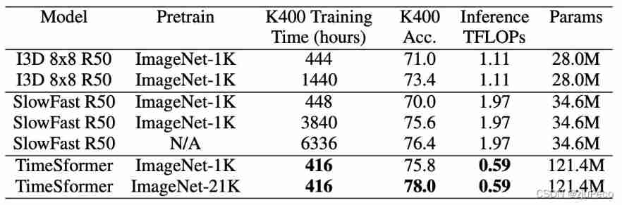
Is space time attention all you need for video understanding?

speech production model

Principle and steps of principal component analysis (PCA)

Paper reading - group normalization

Hstack, vstack and dstack in numpy

Paper reading - jukebox: a generic model for music

Priority queue with dynamically changing priority
随机推荐
03 认识第一个view组件
[reading point paper] deeplobv3+ encoder decoder with Atlas separable revolution
Principle and steps of principal component analysis (PCA)
柏瑞凱電子沖刺科創板:擬募資3.6億 汪斌華夫婦為大股東
Opencv 10 brightness contrast adjustment
[reading some papers] introducing deep learning into the public horizon alexnet
[thoughts in the essay] mourn for development technology expert Mao Xingyun
Opencvsharp4 handwriting recognition
05 tabbar navigation bar function
A real-time target detection model Yolo
Opencv 08 demonstrates the effect of opening and closing operations of erode, dilate and morphological function morphologyex.
Thesis reading - autovc: zero shot voice style transfer with only autoencoder loss
Cumulative tax law: calculate how much tax you have paid in a year
What are the differences in cache/tlb?
OneNote使用指南(一)
Laravel permission export
OpenCVSharpSample04WinForms
Leetcode 450. Delete node in binary search tree [binary search tree]
Classification and summary of system registers in aarch64 architecture of armv8/arnv9
[data and Analysis Visualization] D3 introductory tutorial 1-d3 basic knowledge