当前位置:网站首页>Discrimination gradient descent
Discrimination gradient descent
2022-07-08 02:17:00 【Strawberry sauce toast】
Preface
Gradient descent is the most commonly used deep learning model optimization algorithm . In this paper, the classical gradient descent 、 Stochastic gradient descent 、 Batch random gradient descent is explained separately , Help distinguish the relationship between the three . Finally, take linear regression as an example , According to the optimization results of the model, the characteristics of the three are analyzed .
The full code has been uploaded to :github Complete code
One 、 gradient descent (Gradient Descent, GD)
1.1 The nature of gradient descent
Gradient descent method is a parameter optimization method .
Optimize : It refers to changing parameters x x x To minimize or maximize a function f ( x ) f(x) f(x). Usually , With the most Small turn f ( x ) f(x) f(x) Refers to most optimization problems , Maximization can be transformed from taking the opposite number into minimization , namely m a x x [ f ( x ) ] ⇔ m i n x [ − f ( x ) ] \underset{x}{max}\ [f(x)] \Leftrightarrow \underset{x}{min}\ [-f(x)] xmax [f(x)]⇔xmin [−f(x)].
e.g. The negative log likelihood function is the logarithm of the original likelihood function , Take the opposite number , Transform the maximized likelihood function into the minimized negative log likelihood function .1
1.2 The idea of gradient descent
The basic idea of gradient descent method : Search for the optimal solution along the negative gradient .
Because the direction of negative gradient is the direction in which the value of the function decreases fastest .2
1.3 Calculation of gradient descent
In every iteration , According to the learning rate α \alpha α Update the parameter in the opposite direction of the gradient , Until it converges , The formula is expressed as :
θ ( n + 1 ) = θ ( n ) − α d f d θ ( n ) \theta(n+1)=\theta(n)-\alpha \frac{df}{d\theta (n)} θ(n+1)=θ(n)−αdθ(n)df
Two 、 Deep learning optimization algorithm
Gradient descent is the most commonly used optimization algorithm in deep learning , However, according to the number of samples used for each parameter update , Divided into : Gradient descent method 、 Random gradient descent method 、 Batch random gradient descent method .
2.1 Classic gradient descent method
Suppose that m m m Samples and their labels ( x 1 , y 1 ) , ( x 2 , y 2 ) , . . . , ( x m , y m ) (x_1,y_1),(x_2,y_2),...,(x_m,y_m) (x1,y1),(x2,y2),...,(xm,ym), The predictive value of the model for each sample is y ^ i , i = 1 , 2 , . . . , m \hat y_i,i=1,2,...,m y^i,i=1,2,...,m.
- A single sample ( x i , y i ) (x_i,y_i) (xi,yi) The loss is :
l o s s i ( θ 1 , θ 2 ) = F ( θ 1 , θ 2 ; y i , y ^ i ) loss_i(\theta_1, \theta_2)=F(\theta_1, \theta_2;y_i,\hat y_i) lossi(θ1,θ2)=F(θ1,θ2;yi,y^i)
In style , F ( θ 1 , θ 2 ) F(\theta_1, \theta_2) F(θ1,θ2) Is the loss function of the model , Here the gradient decreases by optimizing the parameters θ 1 , θ 2 \theta_1, \theta_2 θ1,θ2 Minimum loss function .
- The loss function is used to measure the difference between the predicted value of the model and the real value of the sample ;
- In deep learning , Gradient descent method is used for Minimum loss function ;
- The common loss function : Mean square error (Mean Square Error, MSE) Loss 、 Cross entropy (Cross Entropy Loss) Loss .
- The average loss of all samples is :
L o s s ( θ 1 , θ 2 ) = 1 m ∑ i = 1 m l o s s i ( θ 1 , θ 2 ) Loss(\theta_1, \theta_2) = \frac{1}{m}\sum_{i=1}^mloss_i(\theta_1, \theta_2) Loss(θ1,θ2)=m1i=1∑mlossi(θ1,θ2) - Parameters are updated :
For parameters θ 1 \theta_1 θ1: θ 1 ( n + 1 ) = θ 1 ( n ) − α ∂ L o s s ∂ θ 1 \theta_1(n+1)=\theta_1(n)-\alpha \frac{\partial Loss}{\partial \theta_1} θ1(n+1)=θ1(n)−α∂θ1∂Loss
For parameters θ 2 \theta_2 θ2: θ 2 ( n + 1 ) = θ 2 ( n ) − α ∂ L o s s ∂ θ 2 \theta_2(n+1)=\theta_2(n)-\alpha \frac{\partial Loss}{\partial \theta_2} θ2(n+1)=θ2(n)−α∂θ2∂Loss
here , When updating parameters , The average loss of all samples is used .
The classical gradient descent method needs to calculate the loss of all samples every iteration , When the sample size is large (e.g. ImageNet contain 128 Ten thousand training samples ) when , It will consume computing resources , And there are the following deficiencies :
- Slow convergence , Number of iterations required (epoch) many ;
- All training samples are considered at the same time in each calculation , Loss of randomness , It is easy to cause over fitting .
therefore , The idea of random gradient descent came into being .
2.2 Random gradient descent method (Stochasitc Gradient Descent, SGD)
The basic idea of random gradient descent : Calculate the loss of only one sample at a time , Then traverse all samples , Complete a round (epoch) iteration .
Random gradient descent algorithm description :
for epoch in range(epochs): # Run together epochs round
for i in range(m): # Each iteration traverses 1 Samples
L o s s ( θ 1 , θ 2 ) = F ( θ 1 , θ 2 ; y ^ i , y i ) Loss(\theta_1, \theta_2)=F(\theta_1,\theta_2;\hat y_i, y_i) Loss(θ1,θ2)=F(θ1,θ2;y^i,yi) # Calculate the loss of a single sample
θ 1 ( n + 1 ) = θ 1 ( n ) − α ∂ L o s s ∂ θ 1 \theta_1(n+1)=\theta_1(n)-\alpha \frac{\partial Loss}{\partial \theta_1} θ1(n+1)=θ1(n)−α∂θ1∂Loss # Update the parameters with the loss of a single sample
θ 2 ( n + 1 ) = θ 2 ( n ) − α ∂ L o s s ∂ θ 2 \theta_2(n+1)=\theta_2(n)-\alpha \frac{\partial Loss}{\partial \theta_2} θ2(n+1)=θ2(n)−α∂θ2∂Loss
end
end
Compared with the classical gradient descent algorithm, the random gradient descent algorithm has a great improvement in computing speed , But because each iteration only calculates the loss of one sample , The loss fluctuates greatly .
1.3 Batch random gradient decline (mini_batch SGD)
The basic idea of batch random gradient descent : Each iteration selects a small part of the total training sample ( That is, a batch), Calculate the gradient of its average loss to optimize the parameters , Complete the iteration of all training samples as one epoch.
Batch random gradient descent can be described as :
for epoch in range(epochs):
for batch in range(batches):
L o s s ( θ , θ 2 ) = 1 b ∑ i = 1 b F ( θ 1 , θ 2 ; y i , y ^ i ) Loss(\theta, \theta_2)=\frac{1}{b}\sum_{i=1}^bF(\theta_1,\theta_2;y_i,\hat y_i) Loss(θ,θ2)=b1∑i=1bF(θ1,θ2;yi,y^i) # b For one batch Number of samples included
θ 1 ( n + 1 ) = θ 1 ( n ) − α ∂ L o s s ∂ θ 1 \theta_1(n+1)=\theta_1(n)-\alpha \frac{\partial Loss}{\partial \theta_1} θ1(n+1)=θ1(n)−α∂θ1∂Loss # Use one batch The average loss update parameter of the sample
θ 2 ( n + 1 ) = θ 2 ( n ) − α ∂ L o s s ∂ θ 2 \theta_2(n+1)=\theta_2(n)-\alpha \frac{\partial Loss}{\partial \theta_2} θ2(n+1)=θ2(n)−α∂θ2∂Loss
end
end
Compared with random gradient descent , The random gradient descent of batch can alleviate the fluctuation of its loss , Make the calculation result not easy to be affected by a single sample ; Compared with the classic gradient descent , Batch random gradient descent each iteration only calculates the loss of small batch samples , Reduce the occupation of computing resources .
3、 ... and 、 Code implementation
Take linear regression , Use gradient descent 、 Random gradient descent and small batch random gradient descent algorithm optimize model parameters .
3.1 Generate data set
The artificial data set is constructed according to the linear model with noise , The linear model for generating data is :
y = X w + b + ϵ \bold y = \bold X \bold w+\bold b+\bold \epsilon y=Xw+b+ϵ
In style , w , b \bold w, \ \bold b w, b For model parameters , ϵ \bold \epsilon ϵ Is the noise in the sample , Assume that the noise conforms to the mean 0, The variance of 0.5 Is a normal distribution .
''' Generate data set '''
def synthetic_data(w, b, num_examples):
    X = torch.normal(0, 1, (num_examples, len(w)))
    y = torch.matmul(X, w) + b
    y += torch.normal(0, 0.5, y.shape)
    return X, y.reshape((-1,1))
''' Generate data and plot '''
true_w = torch.tensor([3.5])
true_b = 4
features, labels = synthetic_data(true_w, true_b, 1000)
plt.plot(features.numpy(), labels.numpy(), 'b.', label='train data')
true_y = torch.matmul(features, true_w) + true_b
plt.plot(features.numpy(), true_y.reshape((-1,1)).numpy(), 'r-', label='true line')
plt.show()

3.2 Define the regression model
def line_regression(X, w, b):
    return torch.matmul(X, w) + b
3.3 Define the loss function
Use the average variance loss function :
l o s s = 1 2 m ∑ i = 1 m ( y ^ − y ) 2 loss = \frac{1}{2m}\sum_{i=1}^m(\hat y-y)^2 loss=2m1i=1∑m(y^−y)2
In style , m m m The number of samples used for each loss calculation .
def squared_loss(y_hat, y, batch_size):
	""" batch_size = num_examples when , For the classic gradient descent algorithm  batch_size = 1 when , Random gradient descent algorithm  batch_size in range(2, num_examples) when , Random gradient descent for batch  """
    return (y_hat - y.reshape(y_hat.shape)) ** 2 / (2 * batch_size)
3.4 Define optimization algorithms
def sgd_optimizer(params, lr):
    with torch.no_grad():
        for param in params:
            param -= lr * param.grad
            param.grad.zero_()
3.5 model training
''' Initialize model parameters '''
w = torch.normal(0, 0.01, size=(1, 1), requires_grad=True)
b = torch.zeros(1, requires_grad=True)
''' Initialize the super parameter '''
lr = 0.02
num_epochs = 50
batch_size = 50
loss = squared_loss
sgd = sgd_optimizer
net = line_regression
for epoch in range(num_epochs):
    for X, y in data_iter(train_data, train_labels, batch_size):
        l = loss(net(X, w, b), y, batch_size)
        l.sum().backward()
        sgd([w, b], lr)
    with torch.no_grad():
        train_l = loss(net(train_data, w, b), train_labels, len(train_data))
        print('epoch', epoch, ' loss ', float(train_l.sum()))
3.6 Model training results
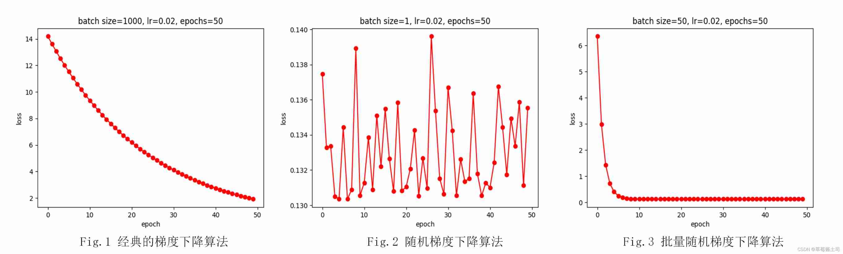
Observing the training result graph can verify the following conclusions 3:
- The classical gradient descent algorithm converges slowly , More iterations are needed epoch To get less loss ;
Self thinking :
We can explain why the classical gradient descent algorithm needs more in terms of the number of parameter updates epochs.
Because the classical gradient descent algorithm needs to calculate the loss of all samples in each iteration , After taking the average value , Back propagation , Update parameters , therefore , Here the parameters are updated ( Back propagation ) The number of times = n u m o f e p o c h s =num\ of\ epochs =num of epochs. And random gradient descent parameter update ( Back propagation ) The number of times = n u m o f e p o c h s × n u m o f e x a m p l e s =num\ of\ epochs \times \ num\ of \ examples =num of epochs× num of examples; Batch random gradient descent parameter update ( Back propagation ) The number of times = n u m o f e p o c h s × n u m o f e x a m p l e s b a t c h s i z e =num \ of \ epochs \times \frac{num\ of \ examples}{batch \ size} =num of epochs×batch sizenum of examples
however epochs The starting point of selection and optimization ( Parameter initialization )、 Selection of learning rate 、 The noise contained in the sample 、 The design of the model and the definition of the loss function are related , Parameters are updated ( Back propagation ) The number of times may be one of the reasons .
- With the same learning rate , The loss of random gradient descent algorithm fluctuates greatly , The result jumps repeatedly around the optimal value ;
- by comparison , Batch random gradient descent converges faster , And the fluctuation is small , But we need to choose the right batch size, And need to weigh batch size And epochs Make the training result 、 The training speed is relatively optimal .
边栏推荐
- burpsuite
- PHP calculates personal income tax
- The bank needs to build the middle office capability of the intelligent customer service module to drive the upgrade of the whole scene intelligent customer service
- Vim 字符串替换
- 牛熊周期与加密的未来如何演变?看看红杉资本怎么说
- Xmeter newsletter 2022-06 enterprise v3.2.3 release, error log and test report chart optimization
- Popular science | what is soul binding token SBT? What is the value?
- LeetCode精选200道--链表篇
- WPF custom realistic wind radar chart control
- Talk about the realization of authority control and transaction record function of SAP system
猜你喜欢

Nanny level tutorial: Azkaban executes jar package (with test samples and results)

What are the types of system tests? Let me introduce them to you

云原生应用开发之 gRPC 入门
Introduction to grpc for cloud native application development

List of top ten domestic industrial 3D visual guidance enterprises in 2022
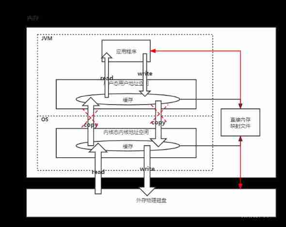
JVM memory and garbage collection-3-direct memory
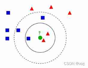
Ml self realization /knn/ classification / weightlessness

Disk rust -- add a log to the program
Leetcode featured 200 channels -- array article

leetcode 865. Smallest Subtree with all the Deepest Nodes | 865.具有所有最深节点的最小子树(树的BFS,parent反向索引map)
随机推荐
PHP calculates personal income tax
Towards an endless language learning framework
image enhancement
VIM use
leetcode 873. Length of Longest Fibonacci Subsequence | 873. 最长的斐波那契子序列的长度
LeetCode精选200道--数组篇
[knowledge map paper] r2d2: knowledge map reasoning based on debate dynamics
See how names are added to namespace STD from cmath file
Introduction to Microsoft ad super Foundation
WPF custom realistic wind radar chart control
Semantic segmentation | learning record (4) expansion convolution (void convolution)
JVM memory and garbage collection-3-object instantiation and memory layout
2022年5月互联网医疗领域月度观察
COMSOL --- construction of micro resistance beam model --- final temperature distribution and deformation --- addition of materials
leetcode 866. Prime Palindrome | 866. prime palindromes
Little knowledge about TXE and TC flag bits
《ClickHouse原理解析与应用实践》读书笔记(7)
List of top ten domestic industrial 3D visual guidance enterprises in 2022
Kwai applet guaranteed payment PHP source code packaging
Talk about the realization of authority control and transaction record function of SAP system