Signal feature extraction +lstm to realize gear reducer fault diagnosis -matlab code

1. Data description

Gearbox data from PHM2009 Data challenge in , Official website ：PHM2009 Data challenge . The tested gears include a set of spur gears and helical gears , In this example, the data of spur gear is used for verification . The photos of the experimental equipment are as follows .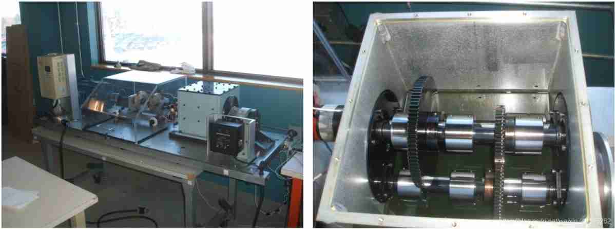


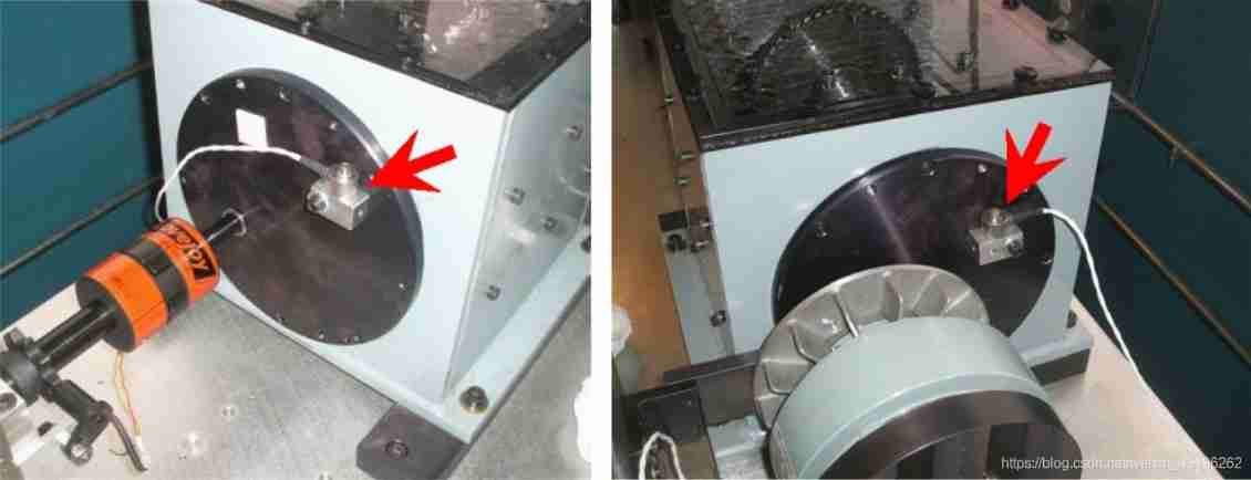
An acceleration sensor is installed on the input side and output side of the gearbox , Sensor parameters ： sensitivity ：10mv/g, Sampling rate 66.67KHz. The acquisition card used collects data from three channels , Respectively :

• passageway 1： Input side vibration sensor data
• passageway 2： Output side vibration sensor data
• passageway 3： Speed signal

Manually inject faults , share 8 Fault types , The following table .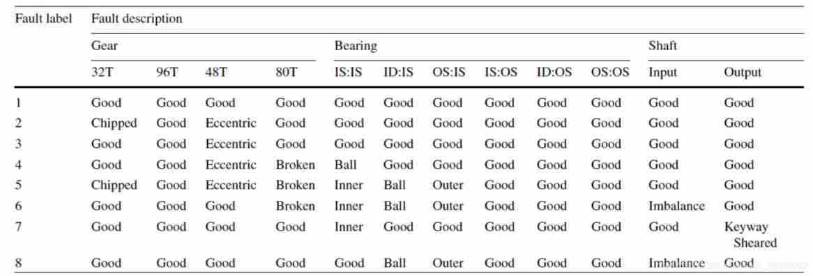

The working condition during the experiment is ： The speed is set to 1800rpm, 2100rpm, 2400rpm, 2700rpm, 3000rpm, The loads are low load and high load respectively , After crossing, there are 10 Three working conditions , Respectively
1800 rpm | Low load ,1800rpm| High load , And so on .
This example uses 1800rpm| High load experimental data modeling and verification , Use channel two, that is, the output side vibration sensor data . Data acquisition of each fault type under each working condition lasts 8 second , So for each fault type , Each channel gets a total of 66.7KHz×8 second =533307 Data points . The data of each fault type is 533307×3 Matrix of channels , The data is in matlab Open as follows .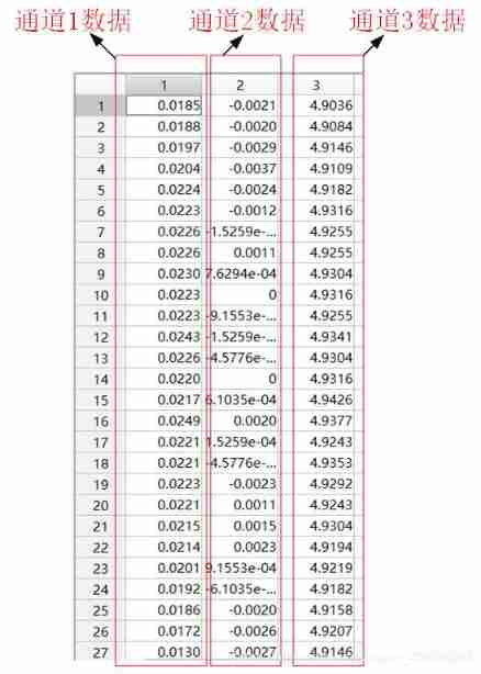

Put the channel 2 The data of plot come out , As shown below .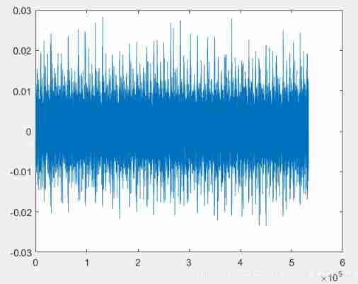

2. Code details

The code consists of two .m file

• read_data_1800_High.m
• main_1800_High.m
  The first one is used to read and divide the original data
  The second one is used to complete the division of training set and test set , feature extraction + Classification, etc

2.1 read_data_1800_High

//  This function Input by 
// interval -  Data partition length , The default is 6400, That is, every 6400 Data points are divided into a sample 
// ind_column -  passageway , The default is 2, That is, select the second channel 
// Output by 
// label1 label2, ..., label8, They are divided into 8 Samples of fault types 
% 
function [label1 label2 label3 label4 label5 label6 label7 label8]= read_data_1800_High( interval, ind_column )
if nargin <2
    ind_column=2; // If the argument passed is less than 2 individual , Default ind_column by 2
end 

if nargin <1
    interval=6400; // Default interval=6400
end

file_rul='E:\Datasets\PHM data challenge\2009 PHM Society Conference Data Challenge-gear box\spur_30hz_High\';
//  Here's how to get file_rul Under the path .mat All files in format 
file_folder=fullfile(file_rul);
dir_output=dir(fullfile(file_folder,'*.mat'));
file_name={
    dir_output.name}';
num_file=max(size(file_name)); //num_file Is the number of files , In this case num_file=8,8 File , Store the... Of the gearbox separately 8 Kinds of fault data 

for i=1:num_file
    file=[file_rul,file_name{
    i}];
    load(file);
    [filepath, name, ext]=fileparts(file);
    raw=eval(name);
    
	//  Every time 6400 Points are divided into one sample 
    n=1;
    left_index=1+(n-1)*interval;
    right_index=n*interval;
    while right_index<=size(raw,1)
         temp=raw(left_index : right_index, ind_column);
         // eval The function structure label1, label2,... And so on 
         eval(['label' num2str(i) '(:,n)=temp;']); 
         n=n+1;
         left_index=1+(n-1)*interval;
         right_index=n*interval;
    end
end
end

2.2 main_1800_High

//  Reading data ,label1 For one 6400*83 Array of ,83 The number of samples obtained for each fault type 
[label1, label2, label3, label4, label5, label6, label7, label8]=read_data_1800_High();
num_categories=8;
//  because matlab in LSTM Modeling requires , use num2cell Function will label1 To cell type ,label_x_cell For one 1×83 Of cell Type of the array , Every cell Storage 6400 Data points 
label1_x_cell=num2cell(label1,1);
label2_x_cell=num2cell(label2,1);
label3_x_cell=num2cell(label3,1);
label4_x_cell=num2cell(label4,1);
label5_x_cell=num2cell(label5,1);
label6_x_cell=num2cell(label6,1);
label7_x_cell=num2cell(label7,1);
label8_x_cell=num2cell(label8,1);

num_1=length(label1_x_cell);
num_2=length(label2_x_cell);
num_3=length(label3_x_cell);
num_4=length(label4_x_cell);
num_5=length(label5_x_cell);
num_6=length(label6_x_cell);
num_7=length(label7_x_cell);
num_8=length(label8_x_cell);
//  Create a data structure for storing labels of each fault type , because matlab in lstm Modeling requires , Also needed cell Type data . for example ,label1_y For one 83×1 Of cell Type of the array , At present, its value is empty 
label1_y=cell(num_1,1);
label2_y=cell(num_2,1);
label3_y=cell(num_3,1);
label4_y=cell(num_4,1);
label5_y=cell(num_5,1);
label6_y=cell(num_6,1);
label7_y=cell(num_7,1);
label8_y=cell(num_8,1);
//  Create a label for the fault type , use 1,2,3,...,8 Express 8 A fault tag , Assign a value to the corresponding tag .
for i=1:num_1; label1_y{
    i}='1'; end
for i=1:num_2; label2_y{
    i}='2'; end
for i=1:num_3; label3_y{
    i}='3'; end
for i=1:num_4; label4_y{
    i}='4'; end
for i=1:num_5; label5_y{
    i}='5'; end
for i=1:num_6; label6_y{
    i}='6'; end
for i=1:num_7; label7_y{
    i}='7'; end
for i=1:num_8; label8_y{
    i}='8'; end
//  use dividerand The function randomly divides the data of each fault type into 4:1 The proportion of , For training and testing respectively 
[trainInd_label1,~,testInd_label1]=dividerand(num_1,0.8,0,0.2);
[trainInd_label2,~,testInd_label2]=dividerand(num_2,0.8,0,0.2);
[trainInd_label3,~,testInd_label3]=dividerand(num_3,0.8,0,0.2);
[trainInd_label4,~,testInd_label4]=dividerand(num_4,0.8,0,0.2);
[trainInd_label5,~,testInd_label5]=dividerand(num_5,0.8,0,0.2);
[trainInd_label6,~,testInd_label6]=dividerand(num_6,0.8,0,0.2);
[trainInd_label7,~,testInd_label7]=dividerand(num_7,0.8,0,0.2);
[trainInd_label8,~,testInd_label8]=dividerand(num_8,0.8,0,0.2);

//  Build training data for each fault type 
xTrain_label1=label1_x_cell(trainInd_label1);
yTrain_label1=label1_y(trainInd_label1);

xTrain_label2=label2_x_cell(trainInd_label2);
yTrain_label2=label2_y(trainInd_label2);

xTrain_label3=label3_x_cell(trainInd_label3);
yTrain_label3=label3_y(trainInd_label3);

xTrain_label4=label4_x_cell(trainInd_label4);
yTrain_label4=label4_y(trainInd_label4);

xTrain_label5=label5_x_cell(trainInd_label5);
yTrain_label5=label5_y(trainInd_label5);

xTrain_label6=label6_x_cell(trainInd_label6);
yTrain_label6=label6_y(trainInd_label6);

xTrain_label7=label7_x_cell(trainInd_label7);
yTrain_label7=label7_y(trainInd_label7);

xTrain_label8=label8_x_cell(trainInd_label8);
yTrain_label8=label8_y(trainInd_label8);

//  Build test data for each fault type 
xTest_label1=label1_x_cell(testInd_label1);
yTest_label1=label1_y(testInd_label1);

xTest_label2=label2_x_cell(testInd_label2);
yTest_label2=label2_y(testInd_label2);

xTest_label3=label3_x_cell(testInd_label3);
yTest_label3=label3_y(testInd_label3);

xTest_label4=label4_x_cell(testInd_label4);
yTest_label4=label4_y(testInd_label4);

xTest_label5=label5_x_cell(testInd_label5);
yTest_label5=label5_y(testInd_label5);

xTest_label6=label6_x_cell(testInd_label6);
yTest_label6=label6_y(testInd_label6);

xTest_label7=label7_x_cell(testInd_label7);
yTest_label7=label7_y(testInd_label7);

xTest_label8=label8_x_cell(testInd_label8);
yTest_label8=label8_y(testInd_label8);

//  Integrate the data of each fault type , Build a complete training set and test set 
xTrain=[xTrain_label1 xTrain_label2 xTrain_label3 xTrain_label4 xTrain_label5 xTrain_label6 xTrain_label7 xTrain_label8];
yTrain=[yTrain_label1; yTrain_label2; yTrain_label3; yTrain_label4; yTrain_label5; yTrain_label6; yTrain_label7; yTrain_label8];
num_train=size(xTrain,2);

xTest=[xTest_label1  xTest_label2  xTest_label3 xTest_label4 xTest_label5 xTest_label6 xTest_label7 xTest_label8];
yTest=[yTest_label1; yTest_label2; yTest_label3; yTest_label4; yTest_label5; yTest_label6; yTest_label7; yTest_label8];
num_test=size(xTest,2);

//================================================================================
// The following is for each sample , Extract three features ：1. Instantaneous frequency ,2. Instantaneous spectral entropy ,3. Wavelet packet energy ,
// The above three features will then be sent to the classifier for classification , Experimental results show that , Take wavelet packet energy as a feature ,
// It can achieve the highest classification accuracy 

//  Extract instantaneous frequency ： use matlab Of pspectrum Perform spectral decomposition on each sample , Reuse instfreq Function to calculate the instantaneous frequency 
FreqResolu=25;
TimeResolu=0.12;
// the output of pspectrum 'p' contains an estimate of the short-term, time-localized power spectrum of x. 
// In this case, p is of size Nf × Nt, where Nf is the length of f and Nt is the length of t.
 [p,f,t]=cellfun(@(x) pspectrum(x,fs,'TimeResolution',TimeResolu,'spectrogram'),xTrain,'UniformOutput', false);
instfreqTrain=cellfun(@(x,y,z) instfreq(x,y,z)', p,f,t,'UniformOutput',false);
[p,f,t]=cellfun(@(x) pspectrum(x,fs,'TimeResolution',TimeResolu,'spectrogram'),xTest,'UniformOutput', false);
instfreqTest=cellfun(@(x,y,z) instfreq(x,y,z)', p,f,t,'UniformOutput',false);

//  Extract instantaneous spectral entropy ： use matlab Of pspectrum Perform spectral decomposition on each sample , Reuse pentropy Function to calculate the instantaneous frequency 
[p,f,t]=cellfun(@(x) pspectrum(x,fs,'TimeResolution',TimeResolu,'spectrogram'),xTrain,'UniformOutput', false);
pentropyTrain=cellfun(@(x,y,z) pentropy(x,y,z)', p,f,t,'UniformOutput',false);
[p,f,t]=cellfun(@(x) pspectrum(x,fs,'TimeResolution',TimeResolu,'spectrogram'),xTest,'UniformOutput', false);
pentropyTest=cellfun(@(x,y,z) pentropy(x,y,z)', p,f,t,'UniformOutput',false);

//  Extract wavelet packet energy 
// num_level=5 Represents the five layer decomposition of wavelet packets , Get... Together 2^5=32 An eigenvector composed of values .
num_level=5; 
index=0:1:2^num_level-1;
// wpdec Is the wavelet packet decomposition function 
treeTrain=cellfun(@(x) wpdec(x,num_level,'dmey'), xTrain, 'UniformOutput', false);
treeTest=cellfun(@(x) wpdec(x,num_level,'dmey'), xTest, 'UniformOutput', false);
for i=1:num_train
    for j=1:length(index)
    	// wprcoef Reconstruct the function for wavelet coefficients 
        reconstr_coef=wprcoef(treeTrain{
    i},[num_level,index(j)]);
        //  Calculate the energy 
        energy(j)=sum(reconstr_coef.^2);
    end
    energyTrain_doule(i,:)=energy;
end

energyTrain=num2cell(energyTrain_doule,2);
energyTrain=energyTrain';

for i=1:num_test
    for j=1:length(index)
        reconstr_coef=wprcoef(treeTest{
    i},[num_level,index(j)]);
        energy(j)=sum(reconstr_coef.^2);
    end
 energyTest_double(i,:)=energy;
end

energyTest=num2cell(energyTest_double,2);
energyTest=energyTest';

// =============== Assemble feature sequences for feeding into the classifier ====================
//  The following statement only uses the wavelet packet energy as the input feature 
xTrainFeature=cellfun(@(x)[x], energyTrain', 'UniformOutput',false);
xTestFeature=cellfun(@(x)[x], energyTest', 'UniformOutput',false);
//  If you want to use   Instantaneous spectral entropy and wavelet packet energy are used as inputs , as follows 
// xTrainFeature=cellfun(@(x,y,z)[x;y;z],energyTrain',instfreqTrain', pentropyTrain', 'UniformOutput',false);
// xTestFeature=cellfun(@(x,y,z)[x;y;z], energyTest',instfreqTest',pentropyTest', 'UniformOutput',false);

// ============================ Data standardization ================================
XV=[xTrainFeature{
    :}];
mu=mean(XV,2);
sg=std(XV,[],2);

xTrainFeatureSD=xTrainFeature;
xTrainFeatureSD=cellfun(@(x)(x-mu)./sg, xTrainFeatureSD,'UniformOutput',false);

xTestFeatureSD=xTestFeature;
xTestFeatureSD=cellfun(@(x)(x-mu)./sg,xTestFeatureSD,'UniformOutput',false);

// ========================= Design LSTM The Internet =================================
yTrain_categorical=categorical(yTrain);
numClasses=numel(categories(yTrain_categorical));
yTest_categorical=categorical(yTest);
sequenceInput=size(xTrainFeatureSD{
    1},1); //  If you chose 3 Features as data , Here instead "3"

//  Create for sequence-to-label Classified LSTM Steps are as follows ：
// 1.  establish sequence input layer
// 2.  Create several LSTM layer
// 3.  Create a fully connected layer
// 4.  Create a softmax layer
// 5.  Create a classification outputlayer
//  Pay attention to sequence input layer Of size Set to the number of feature categories included , In this case ,1 or 2 or 3, Depending on how many features you use .fully connected layer The parameter of is the classification number , In this case 8.
layers = [ ...
    sequenceInputLayer(sequenceInput)
     lstmLayer(256,'OutputMode','last')
    fullyConnectedLayer(numClasses)
    softmaxLayer
    classificationLayer
    ];

maxEpochs=600;
miniBatchSize=32;
//  If you don't want to show the training process ,
options = trainingOptions('adam', ...
    'ExecutionEnvironment', 'gpu',...
     'SequenceLength', 'longest',...
    'MaxEpochs',maxEpochs, ...
    'MiniBatchSize', miniBatchSize, ...
    'InitialLearnRate', 0.001, ...
    'GradientThreshold', 1, ...
    'plots','training-progress', ... 
    'Verbose',true);

// ====================== Training network =========================
net2 = trainNetwork(xTrainFeatureSD,yTrain_categorical,layers,options);
// ====================== Test network ==========================
testPred2 = classify(net2,xTestFeatureSD);
//  Print confusion matrix 
plotconfusion(yTest_categorical',testPred2','Testing Accuracy')

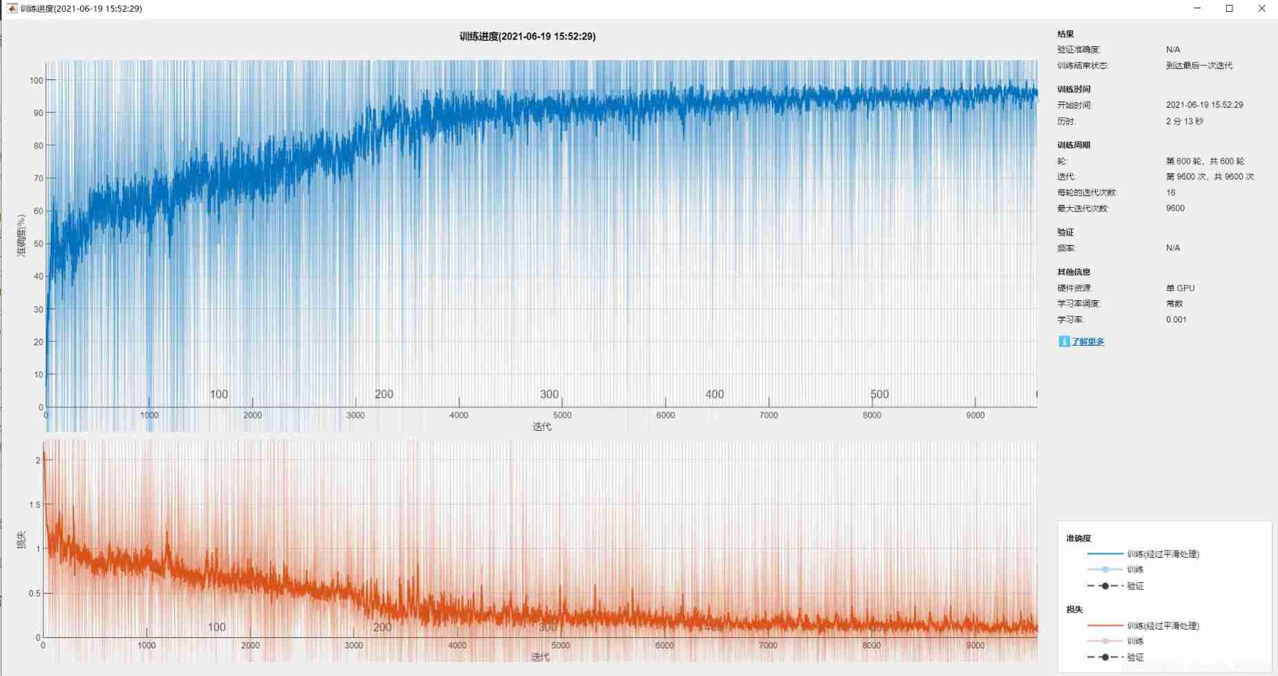
Screenshot of the training process , If you don't want to show this figure , take options Medium 'plots','training-progress', ... Change it to 'plots','none', ...

Screenshot of confusion matrix , You can see , Accuracy of 94%.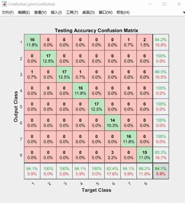

Put the above two files in the same workspace Next , function main_1800_High that will do

3 expectation

In the follow-up study , We found out keras Under the framework of deep learning CNN It's easier to do this kind of problem , Feature extraction is not required , The tutorial will be supplemented later .