当前位置:网站首页>From the perspective of quantitative genetics, why do you get the bride price when you get married
From the perspective of quantitative genetics, why do you get the bride price when you get married
2022-07-05 23:09:00 【Analysis of breeding data】
Betrothal money , It's the money the man gave the woman when he got married . There are two points :
- money
- The man gives the woman
It is said that :“ Father defeat , A setback ; Mother frustration , A nest of frustration ”, It means that a father affects his children , It is a single influence , And the mother affects her children , It is affected by nesting .
because , From a genetic point of view , Children inherit half of their parents' genetic material , But because it is the mother's cytoplasm ( Such as mitochondria ) It also carries genetic material , So mothers pass on more genetic material to their offspring than fathers . therefore , Want to improve the family's genes and personality , Men find a good woman to mate with , Find a better man to mate with than a woman , The impact is greater . Think of it here. , Suddenly I feel married , A lot of betrothal gifts to the woman , It's understandable .
Mother has great influence on offspring , Not just from a genetic point of view ( raw ), And the role of the environment ( Education ), There is also the interaction between genetics and environment ( fertility ). From the perspective of quantitative genetics :
Elementary formula :
Individual performance = Genetic material + Environmental Science ( error )
Advanced formula :
Individual performance = Father's genetic material + Mother's genetic material + Environmental Science ( error )
Further advanced formula :
Individual performance = Father's genetic material + Mother's genetic material + Maternal genetic effects ( Such as mitochondrial genetics )+ Maternal permanent environmental effects ( Such as parenting environment )+ Environmental Science ( error )
In the formula above , Mother provided three :
- Mother's genetic material
- Maternal genetic effects ( Such as mitochondrial genetics )
- Maternal environmental effects ( Such as parenting environment )
Individual permanent environmental effects , Maternal genetic effects , Maternal permanent environmental effects , When building the model , Know it but don't know why , Otherwise One bottle is less than half a bottle The state of is obviously not the quality that a data analyst should have .
1. Several concepts
- Individual permanent environmental effects (Individual permanent environmental effect), Also known as permanent environmental effects , In general, when an individual has a duplicate value, it can be partitioned out , For example, chickens lay eggs , Piglets, etc .
- Maternal genetic effects (Maternal genetic effect), In general, we call the individual additive genetic effect , Because it takes into account the relationship matrix between individuals (A perhaps G perhaps H matrix ), If the matrix is a random factor , Also consider the relationship matrix , It's called maternal genetic effect .
- Maternal environmental effects (Maternal permanent environmental effect), Also known as the maternal permanent environmental effect , As a random factor in analysis , But don't think about the relationship matrix .
2. There are two kinds of maternal effects
The first one is : Maternal genetic effects , There are also two maternal genetic effects , One is to consider the covariance of maternal genetic effect and individual additive effect , One is not to consider , But the default is to consider .
The second kind : Maternal environmental effects , It doesn't take into account the relationship matrix , The model as a random factor .
3. The first one is : Maternal genetic effects
3.1 Consider maternal genetic effects and individual additive effects covariance
Model writing :
y = X b + Z a + Z m g + e y = Xb + Za + Zm_g + e y=Xb+Za+Zmg+e
here :
- Xb Is a fixed factor
- Za Is a random factor , Individual additive effect
- Zm_g Is a random factor , Maternal genetic effects
- e For the residuals
Variance covariance structure :
G = V a r [ a m g ] = [ A σ a 2 A σ a m A σ a m A σ m g 2 ] G = Var\begin{bmatrix} a\\m_g \end{bmatrix} = \begin{bmatrix} A\sigma_a^2 & A\sigma_{am} \\ A\sigma_{am} & A\sigma_{m_g}^2\end{bmatrix} G=Var[amg]=[Aσa2AσamAσamAσmg2]
here A For the relationship matrix , We can see that additive and maternal covariance exist , And both additive and maternal factors need to be considered A matrix .
Example data + Sample code + Sample results
Data and code :
#  Load package
# devtools::install_github("dengfei2013/learnasreml")
library(learnasreml)
# asreml It's commercial software , Need to buy , Please contact :http://www.vsnc.com.cn/
library(asreml)

data("animalmodel.dat")
data("animalmodel.ped")

head(animalmodel.dat)
head(animalmodel.ped)

# m1  The animal model of unisexuality
dat = animalmodel.dat
ped = animalmodel.ped
dat[dat==0] = NA
str(dat)
#  Calculate the inverse relationship matrix
ainv = ainverse(ped)

# m1  The animal model of unisexuality  +  Maternal genetic effects  +  Additive effects interact with maternal genetic effects
m1 = asreml(BWT ~ SEX + BYEAR, random= ~ str(~vm(ANIMAL,ainv) + vm(MOTHER,ainv), ~us(2):vm(ANIMAL,ainv)),
            residual = ~ idv(units),data = dat)
summary(m1)$varcomp
vpredict(m1,h2 ~ V1/(V1+2*V2+V3+V4))
Be careful , there V2 Is the additive and the covariance of the matrix , Because there are two covariances , So when calculating heritability, the denominator should be 2*V2
result :
> summary(m1)$varcomp
                                             component std.error   z.ratio bound %ch
vm(ANIMAL, ainv)+vm(MOTHER, ainv)!us(2)_1:1 1.66469827 0.9069349 1.8355213     P 0.0
vm(ANIMAL, ainv)+vm(MOTHER, ainv)!us(2)_2:1 0.01602755 0.4968458 0.0322586     P 0.8
vm(ANIMAL, ainv)+vm(MOTHER, ainv)!us(2)_2:2 1.35818328 0.4194201 3.2382408     P 0.0
units!units                                 2.19186868 0.6632651 3.3046644     P 0.0
units!R                                     1.00000000        NA        NA     F 0.0
> vpredict(m1,h2 ~ V1/(V1+2*V2+V3+V4))
    Estimate        SE
h2 0.3172785 0.1965149
It can be seen from the results :
- Additive variance components :1.665
- Additive and maternal covariance components :0.016
- Components of maternal genetic variance :1.35
- Residual variance components :2.19
The heritability calculated is 0.317
3.2 Regardless of maternal genetic effects and individual additive effects covariance
Here are two ways to write , The first is to use diag function , Regardless of covariance . The second is to separate additive and maternal genetic effects .
Model writing :
y = X b + Z a + Z m g + e y = Xb + Za + Zm_g + e y=Xb+Za+Zmg+e
here :
- Xb Is a fixed factor
- Za Is a random factor , Individual additive effect
- Zm_g Is a random factor , Maternal genetic effects
- e For the residuals
Variance covariance structure :
G = V a r [ a m g ] = [ A σ a 2 0 0 A σ m g 2 ] G = Var\begin{bmatrix} a\\m_g \end{bmatrix} = \begin{bmatrix} A\sigma_a^2 & 0\\ 0 & A\sigma_{m_g}^2\end{bmatrix} G=Var[amg]=[Aσa200Aσmg2]
here A For the relationship matrix , It can be seen that , Regardless of additive and maternal covariance , And both additive and maternal factors need to be considered A matrix .
Example data + Sample code + Sample results
here , take us Turn into diag, That is, we don't consider covariance .
m2.1 = asreml(BWT ~ SEX + BYEAR, random= ~ str(~vm(ANIMAL,ainv) + vm(MOTHER,ainv), ~diag(2):vm(ANIMAL,ainv)),
            residual = ~ idv(units),data = dat)
summary(m2.1)$varcomp
vpredict(m2.1,h2 ~ V1/(V1+V2+V3))
result :
> summary(m2.1)$varcomp
                                            component std.error  z.ratio bound %ch
vm(ANIMAL, ainv)+vm(MOTHER, ainv)!diag(2)_1  1.689122 0.5291361 3.192225     P 0.0
vm(ANIMAL, ainv)+vm(MOTHER, ainv)!diag(2)_2  1.366709 0.3151848 4.336215     P 0.1
units!units                                  2.174346 0.3932961 5.528523     P 0.0
units!R                                      1.000000        NA       NA     F 0.0
> vpredict(m2.1,h2 ~ V1/(V1+V2+V3))
    Estimate         SE
h2 0.3229569 0.09621066
It can be seen from the results :
- Additive variance components :1.68
- Components of maternal genetic variance :1.36
- Residual variance components :2.17
The heritability calculated is 0.32
Another way of writing :
It can be written in a similar way to additive variance components , Direct use vm function , This kind of writing is relatively simple , But the covariance of additive and maternal genetic effects is not considered .
# m2  The animal model of unisexuality  +  Maternal genetic effects
m2.2 = asreml(BWT ~ SEX + BYEAR, random= ~ vm(ANIMAL,ainv) + vm(MOTHER,ainv),
              residual = ~ idv(units),data = dat)
summary(m2.2)$varcomp
vpredict(m2.2,h2 ~ V1/(V1+V2+V3))
> summary(m2.2)$varcomp
                 component std.error  z.ratio bound %ch
vm(ANIMAL, ainv)  1.689188 0.5292161 3.191868     P   0
vm(MOTHER, ainv)  1.366777 0.3153196 4.334578     P   0
units!units       2.174264 0.3932864 5.528448     P   0
units!R           1.000000        NA       NA     F   0
> vpredict(m2.2,h2 ~ V1/(V1+V2+V3))
    Estimate         SE
h2 0.3229663 0.09621819
You can see that the results are exactly the same .
4. The second kind : Maternal environmental effects
Model writing :
y = X b + Z a + Z m + e y = Xb + Za + Zm + e y=Xb+Za+Zm+e
here :
- Xb Is a fixed factor
- Za Is a random factor , Individual additive effect
- Zm Is a random factor , Maternal environmental effects
- e For the residuals
Variance covariance structure :
G = V a r [ a m g ] = [ A σ a 2 0 0 I σ m g 2 ] G = Var\begin{bmatrix} a\\m_g \end{bmatrix} = \begin{bmatrix} A\sigma_a^2 & 0\\ 0 & I\sigma_{m_g}^2\end{bmatrix} G=Var[amg]=[Aσa200Iσmg2]
here A For the relationship matrix , It can be seen that , Regardless of additive and maternal covariance , And additivity and consideration A matrix , The mother doesn't think about A matrix .
The maternal environmental effect here , Regardless of the kinship matrix , Take it as a random factor .
# m3  The animal model of unisexuality  +  Maternal environmental effects
m3 = asreml(BWT ~ SEX + BYEAR, random= ~ vm(ANIMAL,ainv) + MOTHER,
              residual = ~ idv(units),data = dat)
summary(m3)$varcomp
vpredict(m3,h2 ~ V1/(V1+V2+V3))
result :
> summary(m3)$varcomp
                 component std.error  z.ratio bound %ch
MOTHER            1.104038 0.2398000 4.603997     P   0
vm(ANIMAL, ainv)  2.277785 0.4970861 4.582274     P   0
units!units       1.656900 0.3734446 4.436803     P   0
units!R           1.000000        NA       NA     F   0
> vpredict(m3,h2 ~ V1/(V1+V2+V3))
    Estimate         SE
h2 0.2191107 0.04364284
5. Both maternal genetic effects and maternal environmental effects are considered
This model , It is the most complete model considering maternal effect , He includes
- Maternal genetic effects
- Additive and maternal genetic effect covariance
- Maternal permanent environmental effects
Model writing :
y = X b + Z 1 a + Z 2 m g + Z 3 m e + e y = Xb + Z_1a + Z_2m_g +Z_3m_e + e y=Xb+Z1a+Z2mg+Z3me+e
here :
- Xb Is a fixed factor
- Za Is a random factor , Individual additive effect
- Zm_g Is a random factor , Maternal genetic effects
- Zm Is a random factor , Maternal environmental effects
- e For the residuals
Variance covariance structure :
G = V a r [ a m g m e ] = [ A σ a 2 A σ a m 0 A σ a m A σ m g 2 0 0 0 I σ m e 2 ] G = Var\begin{bmatrix} a\\m_g \\m_e \end{bmatrix} = \begin{bmatrix} A\sigma_a^2 & A\sigma_{am} & 0 \\ A\sigma_{am} & A\sigma_{m_g}^2 & 0 \\0 & 0 & I\sigma_{m_e}^2\end{bmatrix} G=Var⎣⎡amgme⎦⎤=⎣⎡Aσa2Aσam0AσamAσmg2000Iσme2⎦⎤
# m4  The animal model of unisexuality  +  Maternal genetic effects  +  Additive effects interact with maternal genetic effects  +  Maternal environmental effects
m4 = asreml(BWT ~ SEX + BYEAR, random= ~ str(~vm(ANIMAL,ainv) + vm(MOTHER,ainv), ~us(2):vm(ANIMAL,ainv)) + MOTHER,
              residual = ~ idv(units),data = dat)
summary(m4)$varcomp
vpredict(m4,h2 ~ V1/(V1+2*V2+V3+V4+V5))
result :
> summary(m4)$varcomp
                                              component std.error    z.ratio bound %ch
vm(ANIMAL, ainv)+vm(MOTHER, ainv)!us(2)_1:1 1.688055506 0.9091111 1.85681974     P 0.0
vm(ANIMAL, ainv)+vm(MOTHER, ainv)!us(2)_2:1 0.006385884 0.4954503 0.01288905     P 4.0
vm(ANIMAL, ainv)+vm(MOTHER, ainv)!us(2)_2:2 1.057027088 0.4405431 2.39937292     P 0.1
MOTHER                                      0.497693182 0.3694028 1.34729116     P 0.6
units!units                                 2.157268745 0.6628453 3.25455845     P 0.0
units!R                                     1.000000000        NA         NA     F 0.0
> vpredict(m4,h2 ~ V1/(V1+2*V2+V3+V4+V5))
    Estimate        SE
h2 0.3118627 0.1907149
6. Model filtering : The optimal model LRT test
Whether to consider the permanent environmental effect of the mother :m4 VS m1
Whether to consider additive effect and maternal genetic effect covariance :m1 VS m2.1
# LRT test
lrt.asreml(m4,m1,boundary = T)

lrt.asreml(m1,m2.1,boundary = T)
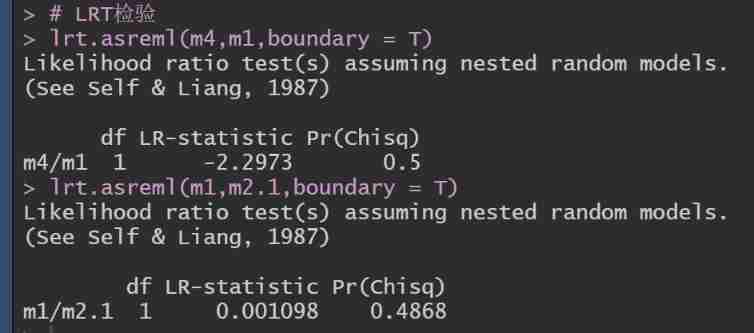
You can see , The maternal permanent environmental effect and covariance are not significant , There can be no .
Which model is the best ? Use BIC Judge :
summary(m1)$bic
summary(m2.1)$bic
summary(m3)$bic
summary(m4)$bic
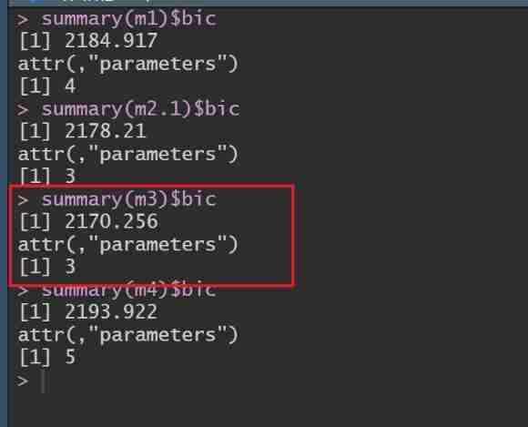
You can see ,m3 Of BIC Minimum , Its model is : Only additive effects and maternal permanent environmental effects are considered .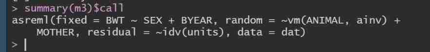
7. Application of genomic selection maternal genetic effects ?
GBLUP perhaps SSGBLUP( One step ) Are the benefits of , Models that can be used in traditional animal models , Genome selection can be done with . Some traits are analyzed , The repeatability model needs to be considered , Maternal inheritance , The mother environment, etc , The analysis will be more accurate .
8. What is the relationship between the above variance components and maternal genetic size ?
We inherit more from the mother than from the father , It also needs data support , For specific traits , Like IQ IQ, For example, height , Such as weight and so on , Which of these traits have greater influence , Which effects are small , We need to use the method of population genetic evaluation to calculate , Then we can draw a conclusion . We are not fortune tellers , We use scientific methods to evaluate and predict .
9. reference
Lawrence R. Schaeffer, Linear Models and Animal Breeding, 2010
A R Gilmour, ASReml User Guide Release 4.1 Structural Specification, 2015
D G Butler, ASReml-R Reference Manual Version, 2018
Finally finished , hurriedly Three companies , give the thumbs-up , Looking at , Hair circle of friends .
边栏推荐
- First, redis summarizes the installation types
- Getting started stm32--gpio (running lantern) (nanny level)
- 东南亚电商指南,卖家如何布局东南亚市场?
- TOPSIS code part of good and bad solution distance method
- Leetcode daily question 1189 The maximum number of "balloons" simple simulation questions~
- audiopolicy
- Use of metadata in golang grpc
- 一文搞定垃圾回收器
- 两数之和、三数之和(排序+双指针)
- Go语言实现原理——锁实现原理
猜你喜欢
终于搞懂什么是动态规划的
傅里叶分析概述

Leetcode weekly The 280 game of the week is still difficult for the special game of the week's beauty team ~ simple simulation + hash parity count + sorting simulation traversal
两数之和、三数之和(排序+双指针)

Three. Js-01 getting started
基于STM32的ADC采样序列频谱分析

Arduino 测量交流电流

d3dx9_ How to repair 31.dll_ d3dx9_ 31. Solution to missing DLL

TypeError: this. getOptions is not a function
Overview of Fourier analysis
随机推荐
Multi sensor fusion of imu/ optical mouse / wheel encoder (nonlinear Kalman filter)
终于搞懂什么是动态规划的
判断二叉树是否为完全二叉树
东南亚电商指南,卖家如何布局东南亚市场?
CJ mccullem autograph: to dear Portland
透彻理解JVM类加载子系统
[digital signal denoising] improved wavelet modulus maxima digital signal denoising based on MATLAB [including Matlab source code 1710]
2022 G3 boiler water treatment simulation examination and G3 boiler water treatment simulation examination question bank
[secretly kill little buddy pytorch20 days] - [Day2] - [example of picture data modeling process]
Global and Chinese markets of industrial pH meters 2022-2028: Research Report on technology, participants, trends, market size and share
Fix the memory structure of JVM in one article
The difference between MVVM and MVC
Nail error code Encyclopedia
TypeError: this. getOptions is not a function
Multi view 3D reconstruction
数学公式截图识别神器Mathpix无限使用教程
Selenium+Pytest自动化测试框架实战
[speech processing] speech signal denoising based on Matlab GUI Hanning window fir notch filter [including Matlab source code 1711]
Yiwen gets rid of the garbage collector
一文搞定JVM常见工具和优化策略