Learn CV two loss function from scratch (1)

notes ： Most of the content of this blog is not original , But I sort out the data I collected before , And integrate them with their own stupid solutions , Convenient for review , All references have been cited , And has been praised and collected ~

Preface ： In deep learning , The loss function plays an important role . Through the loss function, the model can reach the convergence state , Reduce the error of model prediction . therefore , The influence of different loss functions on the model is also different （ One of the daily work of the dispatcher ）. In this chapter , We will explain what is the loss function , Image classification 、 object detection 、 What are the common loss functions of face recognition , What are the specific characteristics ~

1. What is the loss function

In a nutshell , Loss function （loss function） It is used to estimate the predicted value of the model f(x) And the real value Y The degree of inconsistency , It's a non negative real value function , Usually use L(Y, f(x)) To express , The smaller the loss function , The better the robustness of the model .

2. The kind of loss function

2.1 Image classification

2.1.1 Cross entropy loss （Cross Entropy Loss）

For the classification problem , The most commonly used loss function is the cross entropy loss function Cross Entropy Loss, however , The cross entropy loss function can be divided into two application scenarios .

1. II. Classification scenario

Consider two categories , In the second category we usually use Sigmoid Function to compress the output of the model to (0, 1) Within the interval , Since there are only two categories of problems, there are only positive and negative categories （ Yes or no ）, So we also get the probability of negative classes .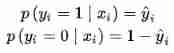

From the perspective of maximum likelihood , The two cases can be combined into one formula ：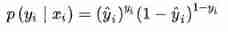

I don't know ？ In fact, it can be seen that
When the real sample label y=0 when , The first term of the above formula ${\left({\hat{y}}_i\right)}^{y_i}$ The value is 1, The probability equation is transformed into :

When the real sample label y=1 when , The second term of the above formula ${\left(1-{\hat{y}}_i\right)}^{1-y_i}$ for 1, The probability equation is transformed into :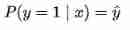

It is the same as the two formulas given at the beginning ！

Suppose the data points are independent and identically distributed , Then the likelihood can be expressed as

Log the likelihood , Then add a minus sign to minimize the negative log likelihood , Is the form of cross entropy loss function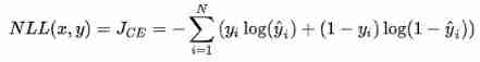

The following figure is a visualization of the cross entropy loss function of two categories , The blue line is the target value of 0 The loss of different outputs , The yellow line is the target value of 1 The loss of time . You can see that the closer you get to the target value loss The smaller it is , As the error increases ,loss Exponential growth .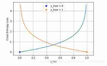

2. Multi category scenarios

In multi category tasks , The derivation of cross entropy loss function is the same as that of binary classification , What changes is the real value y_i Now it's a One-hot vector [4], At the same time, the compression of the model output is changed from the original Sigmoid Replace function with Softmax function （ We said in the last chapter ,sigmoid The function is softmax A special case of , It works softmax Of , It will work sigmoid. Concrete , When the scene becomes binary ,softmax≈sigmoid, Although not rigorous , But it is convenient for everyone to understand ）. Softmax The function limits the output range of each dimension to （0,1） Between , At the same time, the output sum of all dimensions is 1, Used to represent a probability distribution .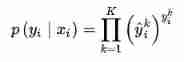

among $k\in K$ Express K One of the categories , The same assumption is that data points are independent and identically distributed , The negative log likelihood can be obtained as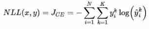

because $y_i$ It's a one-hot vector , Except that the target class is 1 The output on other categories is 0, Therefore, the above formula can also be written as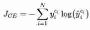

among $c_i$ Is the sample $x_i$ Target class of . Usually, this cross entropy loss function applied to multi classification is also called Softmax Loss perhaps Categorical Cross Entropy Loss.

3. Characteristics of cross entropy loss function

(1) It's also a logarithmic likelihood function in essence , It can be used in binary and multi classification tasks .

(2) When using sigmoid As an activation function , Cross entropy loss function is often used instead of mean square error loss function , Because it can perfectly solve the problem that the weight of the square loss function is updated too slowly , have ” When the error is large , Weight update fast ; When the error is small , Weight update is slow ” Good properties of .

2.1.2 Hinge loss （Hinge Loss）

Hinge loss Hinge Loss Is another two class loss function , Support vector machine Support Vector Machine (SVM) The loss function of the model is essentially Hinge Loss + L2 Regularization . The formula of hinge loss is as follows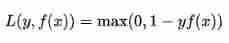

characteristic ：

(1) Hinge Loss It means that if it is classified correctly , The loss is 0, Otherwise, the loss will be $1-yf(x)$ .SVM Is to use this loss function .

(2) General f(x) It's the forecast , stay -1 To 1 Between ,y It's the target value （-1 or 1）, Its meaning is ,f(x) The value of the -1 and +1 Just between , Do not encourage |f(x)| > 1, That is, the classifier is not encouraged to be overconfident , Make a correctly classified sample more than... From the dividing line 1 There will be no reward , Thus, the classifier can focus more on the overall error .

(3) Robustness is relatively high , For outliers 、 Noise is not sensitive , But it doesn't have a very good probability explanation .

5.1.3 0-1 Loss (zero-one loss)

0-1 Loss refers to the fact that the predicted value is not equal to the target value, which is 1, Otherwise 0: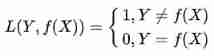

characteristic ：

(1) 0-1 The loss function directly corresponds to the number of classification errors , But it's a nonconvex function .

(2) The perceptron uses this loss function . But the condition of equality is too strict , So you can relax the conditions , The meet $|Y-f(x)|<T$ When you think it's equal , The recent fire RepMlp You can pay attention to .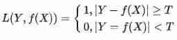

Structure diagram of multilayer perceptron （MLP and CNN Similar structure , but MLP The input is the column vector , and CNN It's a matrix ）：

2.2 object detection

The loss function of target detection task is determined by Classificition Loss and Bounding Box Regeression Loss Two parts make up . The following describes the target detection tasks in recent years Bounding Box Regression Loss Function The evolution of , Its evolution route is Smooth L1 Loss→IoU Loss→GIoU Loss→DIoU Loss→CIoU Loss, This article follows this route .

2.2.1 Smooth L1 Loss

This method was proposed by Microsoft ,Fast RCNN This method is proposed in this paper

hypothesis x Is the difference between the predicted box and the real box , frequently-used L1 and L2 as well as Smooth Loss Defined as ：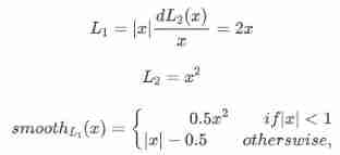

Aforementioned 3 A loss function pair x The derivatives of are ：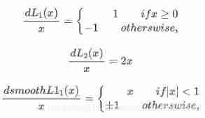

From loss function pair x The derivative of ：
（1） $L_1$ Yes $x$ The derivative of is a constant . This leads to late training , Forecast value and ground truth The difference is very small , The absolute value of the derivative of the loss to the predicted value is still 1, and learning rate If it doesn't change , The loss function will fluctuate near the stable value , It is difficult to continue convergence to achieve higher accuracy .
（2） $x$ When it increases , $L_2$ Loss pair $x$ The derivative of also increases . This leads to early training , Forecast value and groud truth When the difference is too big , The gradient of the loss function to the predicted value is very large , Unstable training .
（3） $Smoot{h}_{L_1}$ stay $x$ More hours , Yes $x$ And the gradient will be smaller , And in the $x$ When a large , Yes $x$ The absolute value of the gradient reaches the upper limit 1, It's not too big to break the network parameters .$Smoot{h}_{L_1}$ Perfectly avoided $L_1$ and $L_2$ Lost defects . The function image is as follows ：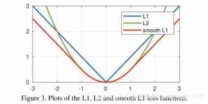

The loss in the regression task of the actual target detection frame loss by

among $v=\left(v_x,v_y,v_w,v_h\right)$ Express GT Frame coordinates of ,$t^u=\left(t_x^u,t_y^u,t_w^u,t_h^u\right)$ Represents the predicted frame coordinates , That is, find 4 Point loss, Then add as Bounding Box Regression Loss.

shortcoming ：

(1) The three above Loss A method for calculating target detection Bounding Box Loss when , Find out independently 4 Point Loss, Then add to get the final Bounding Box Loss, The assumption of this approach is 4 The two points are independent of each other , In fact, there is a certain correlation

(2) The indicator of the actual evaluation box is to use IOU, The two are not equivalent , Multiple check boxes may have the same size $smoot{h}_{L_1}\left(x\right)$ Loss, but IOU It can be very different , In order to solve this problem, we introduced IOU Loss.

2.2.2 Focal Loss

This method was developed by he Kaiming's team in ICCV 2017 Put forward , Thesis link ：

https://arxiv.org/pdf/1708.02002.pdf

Focal loss Mainly to solve one-stage In target detection, the proportion of positive and negative samples is seriously unbalanced . The loss function reduces the weight of a large number of simple negative samples in training , It can also be understood as a kind of difficult sample mining .

Focal loss It is based on the cross entropy loss function , First of all, we review the loss on the intersection of two categories ：

Because it's binary ,p Indicates that the prediction sample belongs to 1 Probability （ The scope is 0-1）,y Express label,y The values for {+1,-1}. When it's true label yes 1, That is to say y=1 when , If a sample x Forecast as 1 The probability of this class p=0.6, So the loss is -log(0.6), Note that the loss is greater than or equal to 0 Of . If p=0.9, So the loss is -log(0.9), therefore p=0.6 The loss is greater than p=0.9 The loss of , It's easy to understand . Let's just take dichotomy as an example , Multi classification and so on .

For convenience , use $p_t$ Instead of p, And the above mentioned p Express True Label Probability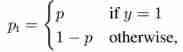

The top formula can be written as ：

Next, we introduce a basic improvement of cross entropy , since one-stage detector When training, there is a big gap between the number of positive and negative samples , Then a common way is to add weight to the positive and negative samples , Negative samples appear more frequently , Then reduce the weight of negative samples , The number of positive samples is small , We should increase the weight of positive samples . So you can set ${\alpha }_t$ To control the sum of positive and negative samples loss The shared weight of .${\alpha }_t$ Take a smaller value to reduce the negative sample （ More samples ） The weight of .

Obviously, the previous formula 3 Although we can control the weight of positive and negative samples , But there is no way to control the weight of easy to classify and difficult to classify samples , So there was Focal Loss：

there $\gamma$ Referred to as focusing parameter, $\gamma >=0$ , and ${\left(1-p_t\right)}^{\gamma }$ It's called modulation coefficient

The purpose of adding modulation coefficient is to reduce the weight of easily classified samples , Thus, the model focuses on the hard to classify samples in training .

The picture below is Focal Loss Compare with the curve of cross entropy function

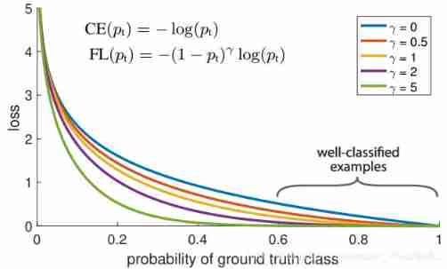
γ=0 Is the standard cross entropy function , It can be seen that ,focal loss It can make the model converge faster

Focal Loss Characteristics ：
（1） When a sample is wrongly divided ,$p_t$ It's very small , So the modulation factor $(1-p_t)$ near 1 , The loss is not affected ; When $p_t\to 1$, factor $（1-p_t）$ near 0, So the score is better （well-classified） The weight of the sample is lowered . So the modulation coefficient tends to 1, That is to say, compared with the original loss There's no big change . When $p_t$ Tend to 1 When （ At this point, the classification is correct and easy to classify samples ）, The modulation coefficient tends to 0, That is, for the total loss My contribution is very small .
（2） When $\gamma =0$ When ,focal loss It's the traditional cross entropy loss , When $\gamma$ When it's added , The modulation coefficient also increases . Focus on the parameters $\gamma$ It smoothly adjusts the proportion of easy to separate samples to lower the weight . $\gamma$ Increase can enhance the influence of modulation factor , It was found that $\gamma$ take 2 best . Intuitively , The modulation factor reduces the loss contribution of easily separated samples , Broaden the range of low loss received by the sample . When $\gamma$ At certain times , For example, equal to 2, Some easy to classify samples $(p_t=0.9)$ Of loss It's better than the standard cross entropy loss Small 100+ times , When $p_t=0.968$ when , smaller 1000+ times , But for hard to classify samples $(p_t<0.5)$,loss It's small at most 4 times . In this case hard example The relative weight has been increased a lot . This reduces the misclassification

The author used the following in the experiment focal loss The formula （ In this way, the weight of positive and negative samples can be adjusted , It can also control the weight of difficult and easy to classify samples ）

Generally speaking, when $\gamma$ When it's added , $\alpha$ It needs to be reduced a little （ In the experiments $\gamma =2$,$\alpha =0.25$ It works best ）

Focal Loss Comparison with other networks ：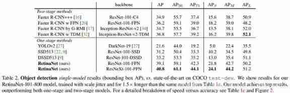

The last line is to use Focal Loss Network of

Reference resources ：

[1] https://zhuanlan.zhihu.com/p/49981234
[2] https://zhuanlan.zhihu.com/p/77686118
[3] https://www.cnblogs.com/dengshunge/p/12252820.html
[4] What is? one-hot vector ？

one-hot Vector is a process of transforming category variables into a form that machine learning algorithms are easy to use , The representation of this vector is the eigenvector of an attribute , That is, there is only one activation point at the same time （ Not for 0）, This vector has only one feature that is not 0 Of , Others are 0, Particularly sparse .
for instance ： One feature “ Gender ”, Gender has “ men ”、“ women ”, This feature has two eigenvalues , There are only two eigenvalues , If this feature is carried out one-hot code , Then the eigenvalue is “ men ” The code of is “10”,“ women ” The code of is “01”, If the eigenvalue has m Discrete eigenvalues , be one-hot The representation of the post eigenvalue is a m Dimension vector , The characteristics of each sample can only have one value , The vector coordinate of this value is 1, Others are 0, If there are multiple characteristics ,“ Gender ” There are two characteristics ,“ Size ”：M、L、XL Three values , We use it “01” For men ,M by “100”,L by “010”,XL by “001”, So a sample ,【“ men ”、"L”】 one-hot Encoded as [10 010], A sample is 5 Dimension vector , This is it. one-hot form .
one-hot The vector is expressed as $t_i=\{0,0,0,\dots ,1,\dots 0\}$ , The length is determined by all discrete eigenvalues of the feature , The number of discrete eigenvalues of all features is added , Generally more than the number of features , The number of specific scene features is different .