当前位置:网站首页>Ml backward propagation
Ml backward propagation
2022-07-08 01:59:00 【xcrj】
neural network
Introduce
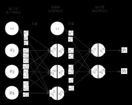
- a n ( l ) a_n^{(l)} an(l):l(layer) The layer number ,n(number) Number , The number of neurons
- w i , j ( l ) w_{i,j}^{(l)} wi,j(l): i = On One layer god the element Ed Number = a n ( l ) Of n i= The number of neurons in the upper layer =a_n^{(l)} Of n i= On One layer god the element Ed Number =an(l) Of n, j = Next One layer god the element Ed Number = a n ( l + 1 ) Of n j= The number of neurons in the next layer =a_n^{(l+1)} Of n j= Next One layer god the element Ed Number =an(l+1) Of n
- w i , j ( l ) w_{i,j}^{(l)} wi,j(l):i,j Represents the position of this element in the matrix ,i On behalf of the line ,j Representative column
- w ( 2 ) = ( w 1 , 1 ( 2 ) w 1 , 2 ( 2 ) w 1 , 3 ( 2 ) w 2 , 1 ( 2 ) w 2 , 2 ( 2 ) w 2 , 3 ( 2 ) w 3 , 1 ( 2 ) w 3 , 2 ( 2 ) w 3 , 3 ( 2 ) ) w^{(2)}=\begin{pmatrix} w_{1,1}^{(2)} & w_{1,2}^{(2)} & w_{1,3}^{(2)} \\ w_{2,1}^{(2)} & w_{2,2}^{(2)} & w_{2,3}^{(2)} \\ w_{3,1}^{(2)} & w_{3,2}^{(2)} & w_{3,3}^{(2)} \end{pmatrix} w(2)=⎝⎜⎛w1,1(2)w2,1(2)w3,1(2)w1,2(2)w2,2(2)w3,2(2)w1,3(2)w2,3(2)w3,3(2)⎠⎟⎞
- w ( 3 ) = ( w 1 , 1 ( 3 ) w 1 , 2 ( 3 ) w 2 , 1 ( 3 ) w 2 , 2 ( 3 ) w 3 , 1 ( 3 ) w 3 , 2 ( 3 ) ) w^{(3)}=\begin{pmatrix} w_{1,1}^{(3)} & w_{1,2}^{(3)} \\ w_{2,1}^{(3)} & w_{2,2}^{(3)} \\ w_{3,1}^{(3)} & w_{3,2}^{(3)} \end{pmatrix} w(3)=⎝⎜⎛w1,1(3)w2,1(3)w3,1(3)w1,2(3)w2,2(3)w3,2(3)⎠⎟⎞
- a n ( l ) = g ( z n ( l ) ) a_n^{(l)}=g(z_n^{(l)}) an(l)=g(zn(l))g yes sigmoid function
- x n = a n ( 1 ) x_n=a_n^{(1)} xn=an(1)
- θ 1 ( 2 ) = w 0 , 1 ( 2 ) , θ 2 ( 2 ) = w 0 , 2 ( 2 ) , θ 3 ( 2 ) = w 0 , 3 ( 2 ) , θ 1 ( 3 ) = w 0 , 1 ( 3 ) , θ 2 ( 3 ) = w 0 , 2 ( 3 ) \theta_1^{(2)}=w_{0,1}^{(2)}, \theta_2^{(2)}=w_{0,2}^{(2)}, \theta_3^{(2)}=w_{0,3}^{(2)}, \theta_1^{(3)}=w_{0,1}^{(3)}, \theta_2^{(3)}=w_{0,2}^{(3)} θ1(2)=w0,1(2),θ2(2)=w0,2(2),θ3(2)=w0,3(2),θ1(3)=w0,1(3),θ2(3)=w0,2(3)
Arithmetic representation :
- a 1 ( 2 ) = g ( z 1 ( 2 ) ) = g ( θ 1 ( 2 ) ∗ 1 + w 1 , 1 ( 2 ) x 1 + w 2 , 1 ( 2 ) x 2 + w 3 , 1 ( 2 ) x 3 ) a_1^{(2)}=g(z_1^{(2)})=g(\theta_1^{(2)}*1+w_{1,1}^{(2)}x_1+w_{2,1}^{(2)}x_2+w_{3,1}^{(2)}x_3) a1(2)=g(z1(2))=g(θ1(2)∗1+w1,1(2)x1+w2,1(2)x2+w3,1(2)x3)
- a 2 ( 2 ) = g ( z 2 ( 2 ) ) = g ( θ 2 ( 2 ) ∗ 1 + w 1 , 2 ( 2 ) x 1 + w 2 , 2 ( 2 ) x 2 + w 3 , 2 ( 2 ) x 3 ) a_2^{(2)}=g(z_2^{(2)})=g(\theta_2^{(2)}*1+w_{1,2}^{(2)}x_1+w_{2,2}^{(2)}x_2+w_{3,2}^{(2)}x_3) a2(2)=g(z2(2))=g(θ2(2)∗1+w1,2(2)x1+w2,2(2)x2+w3,2(2)x3)
- a 3 ( 2 ) = g ( z 3 ( 2 ) ) = g ( θ 3 ( 2 ) ∗ 1 + w 1 , 3 ( 2 ) x 1 + w 2 , 3 ( 2 ) x 2 + w 3 , 3 ( 2 ) x 3 ) a_3^{(2)}=g(z_3^{(2)})=g(\theta_3^{(2)}*1+w_{1,3}^{(2)}x_1+w_{2,3}^{(2)}x_2+w_{3,3}^{(2)}x_3) a3(2)=g(z3(2))=g(θ3(2)∗1+w1,3(2)x1+w2,3(2)x2+w3,3(2)x3)
- a 1 ( 3 ) = g ( z 1 ( 3 ) ) = g ( θ 1 ( 3 ) ∗ 1 + w 1 , 1 ( 3 ) x 1 + w 2 , 1 ( 3 ) x 2 + w 3 , 1 ( 3 ) x 3 ) a_1^{(3)}=g(z_1^{(3)})=g(\theta_1^{(3)}*1+w_{1,1}^{(3)}x_1+w_{2,1}^{(3)}x_2+w_{3,1}^{(3)}x_3) a1(3)=g(z1(3))=g(θ1(3)∗1+w1,1(3)x1+w2,1(3)x2+w3,1(3)x3)
- a 2 ( 3 ) = g ( z 2 ( 3 ) ) = g ( θ 2 ( 3 ) ∗ 1 + w 1 , 2 ( 3 ) x 1 + w 2 , 2 ( 3 ) x 2 + w 3 , 2 ( 3 ) x 3 ) a_2^{(3)}=g(z_2^{(3)})=g(\theta_2^{(3)}*1+w_{1,2}^{(3)}x_1+w_{2,2}^{(3)}x_2+w_{3,2}^{(3)}x_3) a2(3)=g(z2(3))=g(θ2(3)∗1+w1,2(3)x1+w2,2(3)x2+w3,2(3)x3)
- a 1 ( 3 ) = y 1 a_1^{(3)}=y_1 a1(3)=y1
- a 2 ( 3 ) = y 2 a_2^{(3)}=y_2 a2(3)=y2
The matrix represents :
- z ( l ) = w ( l ) a ( l − 1 ) + θ ( l ) z^{(l)}=w^{(l)}a^{(l-1)}+\theta^{(l)} z(l)=w(l)a(l−1)+θ(l), Weight of this layer * The output of the upper layer + The weight of the offset
Forward propagation
Definition
- Input 》 Handle 》 Output , Take the output of the previous layer as the input of the next layer
It is known that
- x ( l ) x^{(l)} x(l) and y y y
- Using forward propagation, we can find : z ( l ) , a ( l ) = g ( z ( l ) ) z^{(l)}, a^{(l)}=g(z^{(l)}) z(l),a(l)=g(z(l))
Back propagation
Introduce
- Backward propagation or reverse propagation is Backward propagation of loss
- MLP Is the loss back propagation and optimization method ( gradient descent ) combination
- Back propagation calculates the gradient of weight in the loss function of neural network , The random gradient descent algorithm uses this gradient for learning
- Machine learning requires computation w w w( The weight ), After defining the loss function , Calculate the loss function w w w( The weight ) Gradient of , The gradient descent algorithm uses this gradient for learning ( to update w w w)
Determine the loss function :
- Mean square error (MSE): C ( w , θ ) = 1 2 ∣ ∣ a ( L ) − y ∣ ∣ 2 2 = 1 2 ∑ i = 1 n ( a i − y i ) 2 C(w,\theta)=\frac{1}{2}||a^{(L)}-y||_2^2=\frac{1}{2}\sum\limits_{i=1}^n(a_i-y_i)^2 C(w,θ)=21∣∣a(L)−y∣∣22=21i=1∑n(ai−yi)2,C yes cost( Cost loss ),L(layer) Said the last 1 layer , a ( L ) a^{(L)} a(L) Is the output layer vector , y y y Is the real output vector , ∣ ∣ x ∣ ∣ 2 ||x||_2 ∣∣x∣∣2 Is a two norm , That's the distance.
Calculate the loss function w w w( The weight ) Gradient of :
One : Calculate the output layer In the loss function w w w( The weight ) Gradient of
- ∂ C ( w , θ ) ∂ w ( L ) = ∂ C ( w , θ ) ∂ a ( L ) ∂ a ( L ) ∂ z ( L ) ∂ z ( L ) ∂ w ( L ) = ( a ( L ) − y ) ⊙ g ( z ( L ) ) ′ a ( L − 1 ) \begin{aligned} \frac{\partial{C(w,\theta)}}{\partial{w^{(L)}}} &=\frac{\partial{C(w,\theta)}}{\partial{a^{(L)}}}\frac{\partial{a^{(L)}}}{\partial{z^{(L)}}}\frac{\partial{z^{(L)}}}{\partial{w^{(L)}}} \\ &=(a^{(L)}-y)\odot g(z^{(L)})^{'}a^{(L-1)} \end{aligned} ∂w(L)∂C(w,θ)=∂a(L)∂C(w,θ)∂z(L)∂a(L)∂w(L)∂z(L)=(a(L)−y)⊙g(z(L))′a(L−1)
- ∂ C ( w , θ ) ∂ θ ( L ) = ∂ C ( w , θ ) ∂ a ( L ) ∂ a ( L ) ∂ z ( L ) ∂ z ( L ) ∂ θ ( L ) = ( a ( L ) − y ) ⊙ g ( z ( L ) ) ′ \begin{aligned} \frac{\partial{C(w,\theta)}}{\partial{\theta^{(L)}}} &=\frac{\partial{C(w,\theta)}}{\partial{a^{(L)}}}\frac{\partial{a^{(L)}}}{\partial{z^{(L)}}}\frac{\partial{z^{(L)}}}{\partial{\theta^{(L)}}} \\ &=(a^{(L)}-y)\odot g(z^{(L)})^{'} \end{aligned} ∂θ(L)∂C(w,θ)=∂a(L)∂C(w,θ)∂z(L)∂a(L)∂θ(L)∂z(L)=(a(L)−y)⊙g(z(L))′
- ⊙ \odot ⊙ yes Hadamaji Hadamard Product, The matrix is multiplied by the corresponding position elements
Two : Count the penultimate 2 layer In the loss function w w w( The weight ) Gradient of
- ∂ C ( w , θ ) ∂ w ( L − 1 ) = ∂ C ( w , θ ) ∂ a ( L ) ∂ a ( L ) ∂ z ( L ) ∂ z ( L ) ∂ a ( L − 1 ) ∂ a ( L − 1 ) ∂ z ( L − 1 ) ∂ z ( L − 1 ) ∂ w ( L − 1 ) = ( a ( L ) − y ) ⊙ g ( z ( L ) ) ′ ⊙ w ( L ) g ( z ( L − 1 ) ) ′ a ( L − 2 ) \begin{aligned} \frac{\partial{C(w,\theta)}}{\partial{w^{(L-1)}}} &=\frac{\partial{C(w,\theta)}}{\partial{a^{(L)}}}\frac{\partial{a^{(L)}}}{\partial{z^{(L)}}}\frac{\partial{z^{(L)}}}{\partial{a^{(L-1)}}}\frac{\partial{a^{(L-1)}}}{\partial{z^{(L-1)}}}\frac{\partial{z^{(L-1)}}}{\partial{w^{(L-1)}}} \\ &=(a^{(L)}-y)\odot g(z^{(L)})^{'}\odot w^{(L)}g(z^{(L-1)})^{'}a^{(L-2)} \end{aligned} ∂w(L−1)∂C(w,θ)=∂a(L)∂C(w,θ)∂z(L)∂a(L)∂a(L−1)∂z(L)∂z(L−1)∂a(L−1)∂w(L−1)∂z(L−1)=(a(L)−y)⊙g(z(L))′⊙w(L)g(z(L−1))′a(L−2)
- ∂ C ( w , θ ) ∂ θ ( L − 1 ) = ∂ C ( w , θ ) ∂ a ( L ) ∂ a ( L ) ∂ z ( L ) ∂ z ( L ) ∂ a ( L − 1 ) ∂ a ( L − 1 ) ∂ z ( L − 1 ) ∂ z ( L − 1 ) ∂ θ ( L − 1 ) = ( a ( L ) − y ) ⊙ g ( z ( L ) ) ′ ⊙ w ( L ) g ( z ( L − 1 ) ) ′ \begin{aligned} \frac{\partial{C(w,\theta)}}{\partial{\theta^{(L-1)}}} &=\frac{\partial{C(w,\theta)}}{\partial{a^{(L)}}}\frac{\partial{a^{(L)}}}{\partial{z^{(L)}}}\frac{\partial{z^{(L)}}}{\partial{a^{(L-1)}}}\frac{\partial{a^{(L-1)}}}{\partial{z^{(L-1)}}}\frac{\partial{z^{(L-1)}}}{\partial{\theta^{(L-1)}}} \\ &=(a^{(L)}-y)\odot g(z^{(L)})^{'}\odot w^{(L)}g(z^{(L-1)})^{'} \end{aligned} ∂θ(L−1)∂C(w,θ)=∂a(L)∂C(w,θ)∂z(L)∂a(L)∂a(L−1)∂z(L)∂z(L−1)∂a(L−1)∂θ(L−1)∂z(L−1)=(a(L)−y)⊙g(z(L))′⊙w(L)g(z(L−1))′
- ∂ C ( w , θ ) ∂ θ ( L ) \frac{\partial{C(w,\theta)}}{\partial{\theta^{(L)}}} ∂θ(L)∂C(w,θ) And ∂ C ( w , θ ) ∂ w ( L − 1 ) \frac{\partial{C(w,\theta)}}{\partial{w^{(L-1)}}} ∂w(L−1)∂C(w,θ) The difference between 3 A formula
3、 ... and : Draw out the public part of No. 1 and No. 2 middle school
- Make δ ( L ) = ∂ C ( w , θ ) ∂ z ( L ) = ( a ( L ) − y ) ⊙ g ( z ( L ) ) ′ \delta^{(L)}=\frac{\partial{C(w,\theta)}}{\partial{z^{(L)}}}=(a^{(L)}-y)\odot g(z^{(L)})^{'} δ(L)=∂z(L)∂C(w,θ)=(a(L)−y)⊙g(z(L))′
- be δ ( L − 1 ) = ∂ C ( w , θ ) ∂ z ( L − 1 ) = ( a ( L ) − y ) ⊙ g ( z ( L ) ) ′ ⊙ w ( L ) g ( z ( L − 1 ) ) ′ \delta^{(L-1)}=\frac{\partial{C(w,\theta)}}{\partial{z^{(L-1)}}}=(a^{(L)}-y)\odot g(z^{(L)})^{'}\odot w^{(L)}g(z^{(L-1)})^{'} δ(L−1)=∂z(L−1)∂C(w,θ)=(a(L)−y)⊙g(z(L))′⊙w(L)g(z(L−1))′
- be δ ( L − 1 ) = δ ( L ) ⊙ w ( L ) g ( z ( L − 1 ) ) ′ \delta^{(L-1)}=\delta^{(L)}\odot w^{(L)}g(z^{(L-1)})^{'} δ(L−1)=δ(L)⊙w(L)g(z(L−1))′
- Then I know δ ( L − 1 ) \delta^{(L-1)} δ(L−1) and δ ( L ) \delta^{(L)} δ(L) The recurrence relation of
Four : Calculate all layers In the loss function w w w( The weight ) Gradient of
The first L layer ( Output layer ) Loss function pair w w w( The weight ) Gradient of :
- ∂ C ( w , θ ) ∂ w ( L ) = δ ( L ) a ( L − 1 ) \frac{\partial{C(w,\theta)}}{\partial{w^{(L)}}}=\delta^{(L)}a^{(L-1)} ∂w(L)∂C(w,θ)=δ(L)a(L−1)
- ∂ C ( w , θ ) ∂ θ ( L ) = δ ( L ) \frac{\partial{C(w,\theta)}}{\partial{\theta^{(L)}}}=\delta^{(L)} ∂θ(L)∂C(w,θ)=δ(L)
The first L-1 layer ( Output layer ) Loss function pair w w w( The weight ) Gradient of :
- ∂ C ( w , θ ) ∂ w ( L − 1 ) = δ ( L − 1 ) a ( L − 2 ) = δ ( L ) ⊙ w ( L ) g ( z ( L − 1 ) ) ′ a ( L − 2 ) \frac{\partial{C(w,\theta)}}{\partial{w^{(L-1)}}}=\delta^{(L-1)}a^{(L-2)}=\delta^{(L)}\odot w^{(L)}g(z^{(L-1)})^{'}a^{(L-2)} ∂w(L−1)∂C(w,θ)=δ(L−1)a(L−2)=δ(L)⊙w(L)g(z(L−1))′a(L−2)
- ∂ C ( w , θ ) ∂ θ ( L − 1 ) = δ ( L − 1 ) = δ ( L ) ⊙ w ( L ) g ( z ( L − 1 ) ) ′ \frac{\partial{C(w,\theta)}}{\partial{\theta^{(L-1)}}}=\delta^{(L-1)}=\delta^{(L)}\odot w^{(L)}g(z^{(L-1)})^{'} ∂θ(L−1)∂C(w,θ)=δ(L−1)=δ(L)⊙w(L)g(z(L−1))′
The first l l l Layer loss function pair w w w( The weight ) Gradient of :
- ∂ C ( w , θ ) ∂ w ( l ) = δ ( l ) a ( l − 1 ) \frac{\partial{C(w,\theta)}}{\partial{w^{(l)}}}=\delta^{(l)}a^{(l-1)} ∂w(l)∂C(w,θ)=δ(l)a(l−1)
- ∂ C ( w , θ ) ∂ θ ( l ) = δ ( l ) \frac{\partial{C(w,\theta)}}{\partial{\theta^{(l)}}}=\delta^{(l)} ∂θ(l)∂C(w,θ)=δ(l)
- ∂ C ( w , θ ) ∂ w ( l − 1 ) = δ ( l − 1 ) a ( l − 2 ) = δ ( l ) ⊙ w ( l ) g ( z ( l − 1 ) ) ′ a ( l − 2 ) \frac{\partial{C(w,\theta)}}{\partial{w^{(l-1)}}}=\delta^{(l-1)}a^{(l-2)}=\delta^{(l)}\odot w^{(l)}g(z^{(l-1)})^{'}a^{(l-2)} ∂w(l−1)∂C(w,θ)=δ(l−1)a(l−2)=δ(l)⊙w(l)g(z(l−1))′a(l−2)
- ∂ C ( w , θ ) ∂ θ ( l − 1 ) = δ ( l − 1 ) = δ ( l ) ⊙ w ( l ) g ( z ( l − 1 ) ) ′ \frac{\partial{C(w,\theta)}}{\partial{\theta^{(l-1)}}}=\delta^{(l-1)}=\delta^{(l)}\odot w^{(l)}g(z^{(l-1)})^{'} ∂θ(l−1)∂C(w,θ)=δ(l−1)=δ(l)⊙w(l)g(z(l−1))′
- know δ ( l ) \delta^{(l)} δ(l) You know ∂ C ( w , θ ) ∂ w ( l ) \frac{\partial{C(w,\theta)}}{\partial{w^{(l)}}} ∂w(l)∂C(w,θ) You know The first l l l Layer loss function pair w w w( The weight ) Gradient of
5、 ... and : summary
It is known that :
- x ( l ) x^{(l)} x(l) and y y y
Forward propagation can be found :
- z ( l ) , a ( l ) = g ( z ( l ) ) z^{(l)}, a^{(l)}=g(z^{(l)}) z(l),a(l)=g(z(l))
Backward propagation can be found :
- δ ( L ) \delta^{(L)} δ(L): because δ ( L ) = ∂ C ( w , θ ) ∂ z ( L ) = ( a ( L ) − y ) ⊙ g ( z ( L ) ) ′ \delta^{(L)}=\frac{\partial{C(w,\theta)}}{\partial{z^{(L)}}}=(a^{(L)}-y)\odot g(z^{(L)})^{'} δ(L)=∂z(L)∂C(w,θ)=(a(L)−y)⊙g(z(L))′ in a ( L ) , y , g ( z ( L ) ) = a ( L ) a^{(L)}, y, g(z^{(L)})=a^{(L)} a(L),y,g(z(L))=a(L) All known
- δ ( L − 1 ) \delta^{(L-1)} δ(L−1): because δ ( L − 1 ) = δ ( L ) ⊙ w ( L ) g ( z ( L − 1 ) ) ′ \delta^{(L-1)}=\delta^{(L)}\odot w^{(L)}g(z^{(L-1)})^{'} δ(L−1)=δ(L)⊙w(L)g(z(L−1))′ in w ( L ) , g ( z ( L − 1 ) ) w^{(L)}, g(z^{(L-1)}) w(L),g(z(L−1)) All known ,== δ ( L ) \delta^{(L)} δ(L)== It can be seen from the above that
- δ ( L − 2 ) \delta^{(L-2)} δ(L−2): because δ ( L − 2 ) = δ ( L − 1 ) ⊙ w ( L − 1 ) g ( z ( L − 2 ) ) ′ \delta^{(L-2)}=\delta^{(L-1)}\odot w^{(L-1)}g(z^{(L-2)})^{'} δ(L−2)=δ(L−1)⊙w(L−1)g(z(L−2))′ in w ( L − 1 ) , g ( z ( L − 2 ) ) w^{(L-1)}, g(z^{(L-2)}) w(L−1),g(z(L−2)) All known ,== δ ( L − 1 ) \delta^{(L-1)} δ(L−1)== It can be seen from the above that
- δ ( l − 1 ) \delta^{(l-1)} δ(l−1): because δ ( l − 1 ) = δ ( l ) ⊙ w ( l ) g ( z ( l − 1 ) ) ′ \delta^{(l-1)}=\delta^{(l)}\odot w^{(l)}g(z^{(l-1)})^{'} δ(l−1)=δ(l)⊙w(l)g(z(l−1))′ in w ( l ) , g ( z ( l − 1 ) ) w^{(l)}, g(z^{(l-1)}) w(l),g(z(l−1)) All known ,== δ ( l ) \delta^{(l)} δ(l)== It can be seen from the above that
- ∂ C ( w , θ ) ∂ w ( L ) = δ ( L ) a ( L − 1 ) \frac{\partial{C(w,\theta)}}{\partial{w^{(L)}}}=\delta^{(L)}a^{(L-1)} ∂w(L)∂C(w,θ)=δ(L)a(L−1)
- ∂ C ( w , θ ) ∂ θ ( L ) = δ ( L ) \frac{\partial{C(w,\theta)}}{\partial{\theta^{(L)}}}=\delta^{(L)} ∂θ(L)∂C(w,θ)=δ(L)
- ∂ C ( w , θ ) ∂ w ( L − 1 ) = δ ( L − 1 ) a ( L − 2 ) \frac{\partial{C(w,\theta)}}{\partial{w^{(L-1)}}}=\delta^{(L-1)}a^{(L-2)} ∂w(L−1)∂C(w,θ)=δ(L−1)a(L−2)
- ∂ C ( w , θ ) ∂ θ ( L − 1 ) = δ ( L − 1 ) \frac{\partial{C(w,\theta)}}{\partial{\theta^{(L-1)}}}=\delta^{(L-1)} ∂θ(L−1)∂C(w,θ)=δ(L−1)
- ∂ C ( w , θ ) ∂ w ( L − 2 ) = δ ( L − 2 ) a ( L − 3 ) \frac{\partial{C(w,\theta)}}{\partial{w^{(L-2)}}}=\delta^{(L-2)}a^{(L-3)} ∂w(L−2)∂C(w,θ)=δ(L−2)a(L−3)
- ∂ C ( w , θ ) ∂ θ ( L − 2 ) = δ ( L − 1 ) \frac{\partial{C(w,\theta)}}{\partial{\theta^{(L-2)}}}=\delta^{(L-1)} ∂θ(L−2)∂C(w,θ)=δ(L−1)
- ∂ C ( w , θ ) ∂ w ( l ) = δ ( l ) a ( l − 1 ) \frac{\partial{C(w,\theta)}}{\partial{w^{(l)}}}=\delta^{(l)}a^{(l-1)} ∂w(l)∂C(w,θ)=δ(l)a(l−1)
- ∂ C ( w , θ ) ∂ θ ( l ) = δ ( l ) \frac{\partial{C(w,\theta)}}{\partial{\theta^{(l)}}}=\delta^{(l)} ∂θ(l)∂C(w,θ)=δ(l)
summary
- Clear purpose : Calculate the weight w w w And offset θ \theta θ( y = a x + b , z = w x + θ , a = g ( z ) = g ( w x + θ ) y=ax+b, z=wx+\theta, a=g(z)=g(wx+\theta) y=ax+b,z=wx+θ,a=g(z)=g(wx+θ))
- initialization w , θ w, \theta w,θ
- Forward propagation calculation z ( l ) , a ( l ) z^{(l)}, a^{(l)} z(l),a(l)
- Define the loss function - Mean square error (MSE) C ( w , θ ) = 1 2 ∣ ∣ a ( L ) − y ∣ ∣ 2 2 = 1 2 ∑ i = 1 n ( a i − y i ) 2 C(w,\theta)=\frac{1}{2}||a^{(L)}-y||_2^2=\frac{1}{2}\sum\limits_{i=1}^n(a_i-y_i)^2 C(w,θ)=21∣∣a(L)−y∣∣22=21i=1∑n(ai−yi)2
- Calculate the output layer (L layer ) Of δ ( L ) \delta^{(L)} δ(L)
- δ ( L ) = ∂ C ( w , θ ) ∂ z ( L ) = ( a ( L ) − y ) ⊙ g ( z ( L ) ) ′ \delta^{(L)}=\frac{\partial{C(w,\theta)}}{\partial{z^{(L)}}}=(a^{(L)}-y)\odot g(z^{(L)})^{'} δ(L)=∂z(L)∂C(w,θ)=(a(L)−y)⊙g(z(L))′
- Backward propagation calculation l l l Layer of δ ( l ) , l = 2 , . . . , L − 1 \delta^{(l)}, l=2,...,L-1 δ(l),l=2,...,L−1
- Using machine learning methods - The gradient descent algorithm updates the weight w w w And offset θ \theta θ
- w ( l ) = w ( l ) − α ∂ C ( w , θ ) ∂ w ( l ) w^{(l)}=w^{(l)}-\alpha \frac{\partial{C(w,\theta)}}{\partial{w^{(l)}}} w(l)=w(l)−α∂w(l)∂C(w,θ)
- θ ( l ) = θ ( l ) − α ∂ C ( w , θ ) ∂ θ ( l ) \theta^{(l)}=\theta^{(l)}-\alpha \frac{\partial{C(w,\theta)}}{\partial{\theta^{(l)}}} θ(l)=θ(l)−α∂θ(l)∂C(w,θ)
- if w , θ w, \theta w,θ The change of is less than the given threshold ( Express w , θ w, \theta w,θ No more changes ) Or the number of iterations , Exit iteration
- Output w , θ w, \theta w,θ
边栏推荐
- 【错误】加载h5权重出错AttributeError: ‘str‘ object has no attribute ‘decode‘
- 图解网络:揭开TCP四次挥手背后的原理,结合男女朋友分手的例子,通俗易懂
- The body has a mysterious margin of 8px
- List of top ten domestic industrial 3D visual guidance enterprises in 2022
- Application of slip ring in direct drive motor rotor
- 进程和线程的退出
- Cross modal semantic association alignment retrieval - image text matching
- C语言-Cmake-CMakeLists.txt教程
- Tencent game client development interview (unity + cocos) double bombing social recruitment 6 rounds of interviews
- From starfish OS' continued deflationary consumption of SFO, the value of SFO in the long run
猜你喜欢
静态路由配置全面详解,静态路由快速入门指南
![[SolidWorks] modify the drawing format](/img/3c/b00e4510b1e129069140c2666c0727.png)
[SolidWorks] modify the drawing format
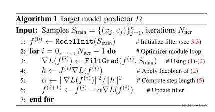
【目标跟踪】|DiMP: Learning Discriminative Model Prediction for Tracking

第七章 行为级建模

The function of carbon brush slip ring in generator
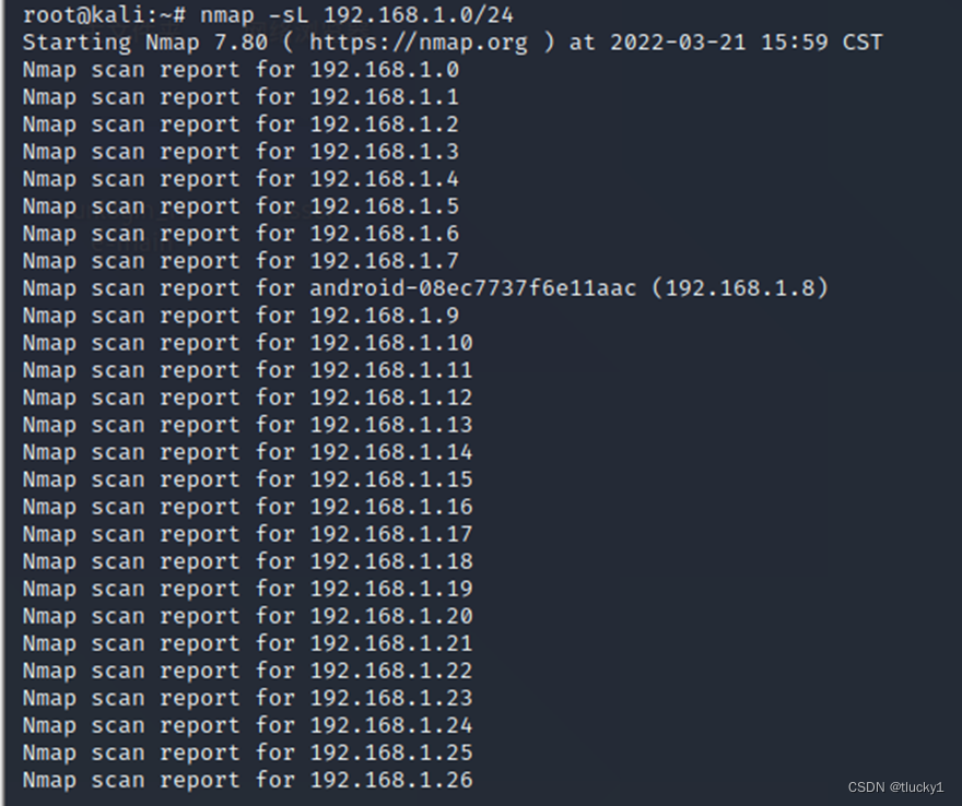
nmap工具介紹及常用命令

很多小夥伴不太了解ORM框架的底層原理,這不,冰河帶你10分鐘手擼一個極簡版ORM框架(趕快收藏吧)

From starfish OS' continued deflationary consumption of SFO, the value of SFO in the long run
SQLite3 data storage location created by Android
软件测试笔试题你会吗?

随机推荐
List of top ten domestic industrial 3D visual guidance enterprises in 2022
From starfish OS' continued deflationary consumption of SFO, the value of SFO in the long run
PHP 计算个人所得税
How to fix the slip ring
Why does the updated DNS record not take effect?
Tapdata 的 2.0 版 ,开源的 Live Data Platform 现已发布
nmap工具介紹及常用命令
Tapdata 的 2.0 版 ,開源的 Live Data Platform 現已發布
WPF 自定义 写实风 雷达图控件
【SolidWorks】修改工程图格式
关于TXE和TC标志位的小知识
城市土地利用分布数据/城市功能区划分布数据/城市poi感兴趣点/植被类型分布
burpsuite
很多小夥伴不太了解ORM框架的底層原理,這不,冰河帶你10分鐘手擼一個極簡版ORM框架(趕快收藏吧)
DataWorks值班表
In depth analysis of ArrayList source code, from the most basic capacity expansion principle, to the magic iterator and fast fail mechanism, you have everything you want!!!
快速熟知XML解析
Partage d'expériences de contribution à distance
Applet running under the framework of fluent 3.0
#797div3 A---C