Program simulation perceptron algorithm (gradient descent method sklearn.linear_ Perception method in model)

Want to make APP Same thing as WeChat , Can run small programs smoothly ？ | Experience will send you to Xinjiang 、 Huawei 、 Cherry keyboard ！>>>

Chapter two The original form simulation of the perceptron

• I'm Xiaobai ; This article code reprint address, there is a note at the end of the article ; Most of the notes are written by themselves , If you have any questions, please give me more advice .

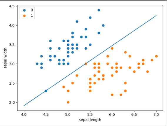
1. Simulated perceptron algorithm by gradient descent . The data comes from sklearn.datasets The classic dataset in the middle of .

import numpy as np
import pandas as pd
#  Import dataset load_iris.
#  The first four columns are calyx length , Calyx width , Petal length , Petal width, etc 4 Attributes used to identify iris ,
from sklearn.datasets import load_iris
import matplotlib.pyplot as plot

# load data
iris = load_iris()

#  Constructors DataFrame(data,index,columns),data For data ,index Index rows ,columns Index columns 
#  Construct data structures 
df = pd.DataFrame(data=iris.data, columns=iris.feature_names)

#  stay df A new column has been added to ： Name label The data of target, That's the type 
#  The first 5 In the category of iris （ Include Setosa,Versicolour,Virginica Three types of ）.
#  That is, by determining the calyx length , Calyx width , Petal length , The size of the petal width is used to identify the type of iris .
df['label'] = iris.target
df.columns = ['sepal length', 'sepal width', 'petal length', 'petal width', 'label']

#  Print out label The number of column values . And column name 、 type 
# print(df.label.value_counts())

#  Create array ,
#  The first parameter :100 It means take 0-99 That's ok , The former 100 That's ok ; Empathy 100： After 100 That's ok .
#  The second parameter ,0,1 For the first and second columns ,-1 It means the last column 
data = np.array(df.iloc[:100, [0, 1, -1]])

#  Array cutting ,X Cut out the last column ;y Cut only the last column 
X, y = data[:, :-1], data[:, -1]

#  Data collation , take y Central African 1 Of is changed to -1
y = np.array([1 if i == 1 else -1 for i in y])

#  The data are linearly separable , Two categories of data 
#  Here is a linear equation of one variable 
class Model:
    def __init__(self):
        # w It starts with the same number of independent variables （1,1） front 
        self.w = np.ones(len(data[0]) - 1, dtype=np.float32)
        self.b = 0
        #  The learning rate is set to 0.1
        self.l_rate = 0.1

    def sign(self, x, w, b):
        # dot The function is a dot product , The difference in * ride .
        # dot Matrix multiplication is the operation of matrix , One row by one column .
        # * When you're doing matrix multiplication , It's the multiplication of the corresponding elements 
        y = np.dot(x, w) + b
        return y

    #  Random gradient descent method 
    def fit(self, X_train, y_train):
        is_wrong = False
        while not is_wrong:
            #  Record the number of points of current classification errors , When the number of misclassification points returns to zero , That's the end of classification 
            wrong_count = 0
            # d from 0-49 Traverse 
            for d in range(len(X_train)):
                #  there X For a row two column array 
                X = X_train[d]
                y = y_train[d]
                if y * self.sign(X, self.w, self.b) <= 0:
                    self.w = self.w + self.l_rate * np.dot(y, X)
                    self.b = self.b + self.l_rate * y
                    wrong_count += 1
            if wrong_count == 0:
                is_wrong = True
        return 'Perceptron Model!'

    def score(self):
        pass

perceptron = Model()
#  Yes perception Make a gradient descent 
perceptron.fit(X, y)

print(perceptron.w)
x_points = np.linspace(4, 7, 10)
#  The final fitting function is as follows ：
# w1*x1 + w2*x2 + b = 0
#  among x1 It's the one below x_points,x2 Namely y_
y_ = -(perceptron.w[0] * x_points + perceptron.b) / perceptron.w[1]
plot.plot(x_points, y_)

# scatter The two properties correspond to x,y.
#  First draw the front 50 Calyx length and width of each point , The flower type is 0;
#  And then draw 50-100, Now the flower type 1
plot.scatter(df[:50]['sepal length'], df[:50]['sepal width'], label='0')
plot.scatter(df[50:100]['sepal length'], df[50:100]['sepal width'], label='1')
#  Abscissa name 
plot.xlabel('sepal length')
#  Ordinate name 
plot.ylabel('sepal width')
plot.legend()
plot.show()

The result is shown in Fig.

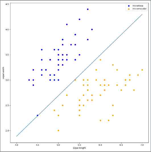
2. sklearn A ready-made perceptron method is provided in , We can call

import sklearn
import pandas as pd
import numpy as np
import matplotlib.pyplot as plt
from sklearn.datasets import load_iris
from sklearn.linear_model import Perceptron

iris = load_iris()
df = pd.DataFrame(iris.data, columns=iris.feature_names)
df['label'] = iris.target
# df.columns = [
#     'sepal length', 'sepal width', 'petal length', 'petal width', 'label'
# ]
data = np.array(df.iloc[:100, [0, 1, -1]])
X, y = data[:, :-1], data[:, -1]
y = np.array([1 if i == 1 else -1 for i in y])

clf = Perceptron(fit_intercept=True,  # true Represents the estimated intercept 
                 max_iter=1000,  #  The maximum number of training data 
                 shuffle=True,  #  Whether to retrain after each training 
                 tol=None)  #  If not set none Then the iteration will be less than 1e-3 end 
clf.fit(X, y)

#  Output after bonding w
print(clf.coef_)
#  Output the intercept after fitting b
print(clf.intercept_)

#  Canvas size 
plt.figure(figsize=(10, 10))

#  Chinese title 
# plt.rcParams['font.sans-serif'] = ['SimHei']
# plt.rcParams['axes.unicode_minus'] = False
# plt.title(' Iris linear data example ')

plt.scatter(data[:50, 0], data[:50, 1], c='b', label='Iris-setosa',)
plt.scatter(data[50:100, 0], data[50:100, 1], c='orange', label='Iris-versicolor')

#  Draw the wires of the sensor 
x_ponits = np.arange(4, 8)
y_ = -(clf.coef_[0][0]*x_ponits + clf.intercept_)/clf.coef_[0][1]
plt.plot(x_ponits, y_)

#  Other parts 
plt.legend()  #  Show Legend 
plt.grid(False)  #  Don't show grid 
plt.xlabel('sepal length')
plt.ylabel('sepal width')
plt.legend()
plt.show()

The result is shown in Fig.