当前位置:网站首页>Skimage learning (3) -- adapt the gray filter to RGB images, separate colors by immunohistochemical staining, and filter the maximum value of the region
Skimage learning (3) -- adapt the gray filter to RGB images, separate colors by immunohistochemical staining, and filter the maximum value of the region
2022-07-07 17:02:00 【Original knowledge】
1、 Adapt the grayscale filter RGB Images
There are many filters for gray images rather than color images . In order to simplify the creation, it can adapt RGB The process of image function ,scikit-image Provides adapt_rgb Decorator .
To actually use adapt_rgb Decorator , You must decide how to adjust RGB Images , For use with grayscale filters . There are two predefined handlers :
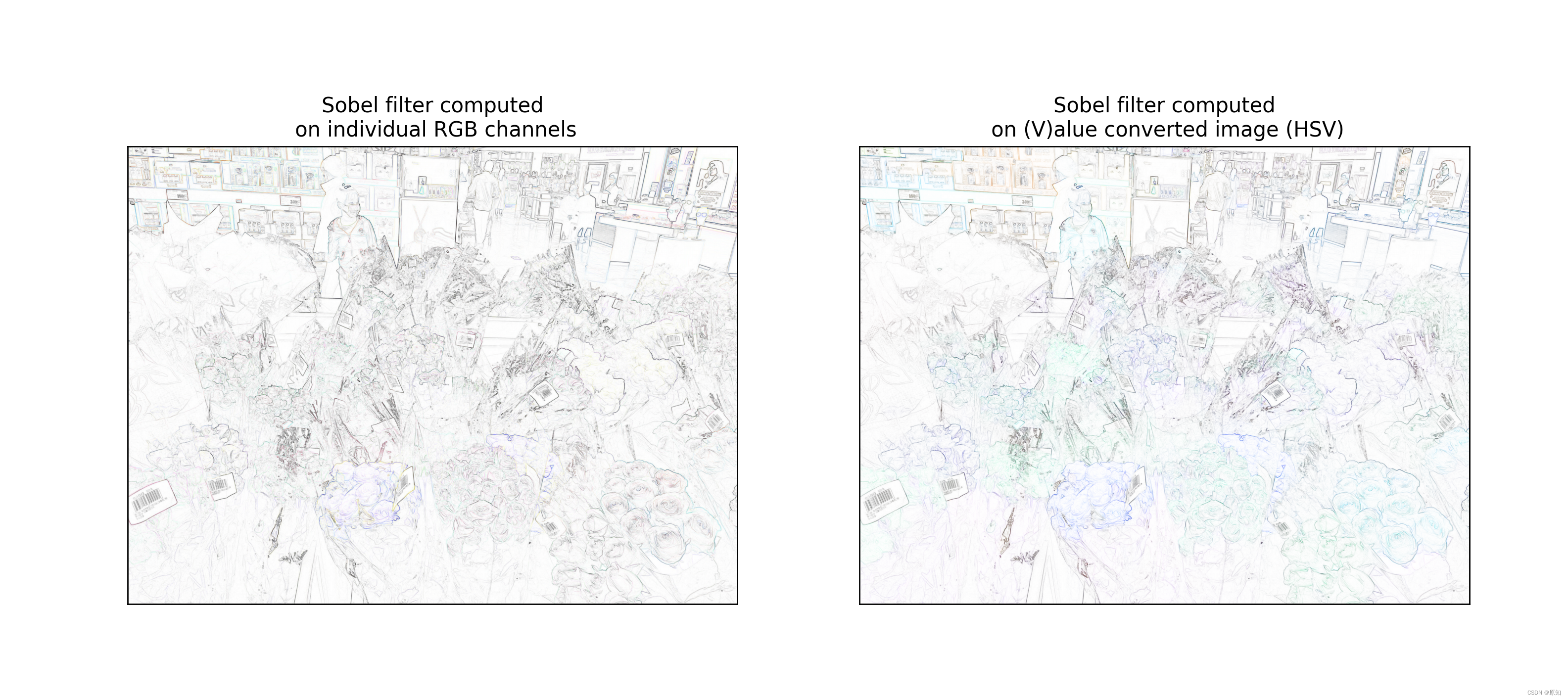
each_channel: Each one RGB The channels are passed to the filter one by one , Then sew the result back RGB Image .
hsv_value: take RGB Image to HSV, And pass the value channel to the filter . The filtered results are inserted into HSV Image , And convert back to RGB.
import skimage
from skimage.color.adapt_rgb import adapt_rgb, each_channel, hsv_value
from skimage import filters
''' General filters are for gray-scale images ,scikit-image Library provides for color image filtering decorator: adapt_rgb,adapt_rgb Two forms of filtering are provided , One is right rgb The three channels are processed separately , Another way is to rgb To hsv Color model , And then for v Channel processing , Finally, turn back to rgb Color model . https://blog.csdn.net/weixin_30244681/article/details/95619723 '''
@adapt_rgb(each_channel)
def sobel_each(image):
return filters.sobel(image)# Use Sobel The filter finds edges in the image .
@adapt_rgb(hsv_value)
def sobel_hsv(image):
return filters.sobel(image)
# We can use these functions as usual , But now they can process gray-scale images and color images at the same time . Let's draw the results with color images :
from skimage import data
from skimage.exposure import rescale_intensity
import matplotlib.pyplot as plt
#image = data.astronaut()
image=skimage.io.imread('11.jpg',)
fig, (ax_each, ax_hsv) = plt.subplots(ncols=2, figsize=(14, 7))
# We use 1 - sobel_each(image), But if the image is not standardized , It will not work
ax_each.imshow(rescale_intensity(1 - sobel_each(image)))# The meaning of this sentence ?, I guess it is to adjust the right rgb Filtering of three channels , And show pictures
''' rescale_intensity: Return to the image after stretching or reducing its intensity level . Strength range required for input and output ,in_range and out_range Used to stretch or narrow the intensity range of the input image . See the example below . '''
ax_each.set_xticks([]), ax_each.set_yticks([])# Set... With scale list x、y scale
ax_each.set_title("Sobel filter computed\n on individual RGB channels")
''' Adjust the intensity function :skimage.exposure.rescale_intensity(image, in_range='image', out_range='dtype') in_range: Indicates the intensity range of the input picture , The default is 'image', Represents the maximum size of the image / The minimum pixel value is used as the range out_range: Indicates the intensity range of the output picture , The default is 'dype', Represents the maximum of the type of image used / The minimum value is used as the range By default , Enter the name of the picture [min,max] The range is stretched to [dtype.min, dtype.max], If dtype=uint8, that dtype.min=0, dtype.max=255 '''
''' matplotlib Library axiss Module Axes.set_xticks() The function is used to set x scale . usage : Axes.set_xticks(self, ticks, minor=False) Parameters : This method accepts the following parameters . ticks: This parameter is x List of axis scale positions . minor: This parameter is used to set the primary or secondary tick marks Return value : This method does not return any value . '''
# We use 1 - sobel_hsv(image) but this won't work if image is not normalized
ax_hsv.imshow(rescale_intensity(1 - sobel_hsv(image)))
ax_hsv.set_xticks([]), ax_hsv.set_yticks([])
ax_hsv.set_title("Sobel filter computed\n on (V)alue converted image (HSV)")
''' Be careful , The result of the value filtered image retains the color of the original image , But the images filtered by the channel are combined in a more surprising way . In other common cases , For example, smooth , The channel filtered image will produce better results than the filtered image . You can also for adapt_rgb Create your own handler function . So , Just create a function with the following signature '''
def handler(image_filter, image, *args, **kwargs):
# Manipulate RGB image here...
image = image_filter(image, *args, **kwargs)
# Manipulate filtered image here...
return image
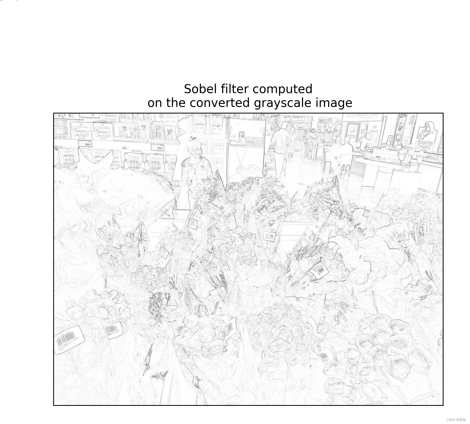
''' Be careful ,adapt_rgb The handler is written for the filter whose image is the first parameter . As a very simple example , We can take any RGB The image is converted to grayscale , Then return the filtered results : '''
from skimage.color import rgb2gray
def as_gray(image_filter, image, *args, **kwargs):
gray_image = rgb2gray(image)# take RGB The image is converted to grayscale
return image_filter(gray_image, *args, **kwargs)
''' Create a use *args and **kwargs It is important to pass the signature of the parameter to the filter , In this way, the modified function can have any number of position and keyword parameters . Last , We can be as right as before adapt_rgb Use this handler : '''
# Gray filtering
@adapt_rgb(as_gray)
def sobel_gray(image):
return filters.sobel(image)
fig, ax = plt.subplots(ncols=1, nrows=1, figsize=(7, 7))
# We use 1 - sobel_gray(image) but this won't work if image is not normalized
ax.imshow(rescale_intensity(1 - sobel_gray(image)), cmap=plt.cm.gray)
ax.set_xticks([]), ax.set_yticks([])
ax.set_title("Sobel filter computed\n on the converted grayscale image")
plt.show()
2、 Immunohistochemical staining separates colors
Color deconvolution refers to the color separation of features .
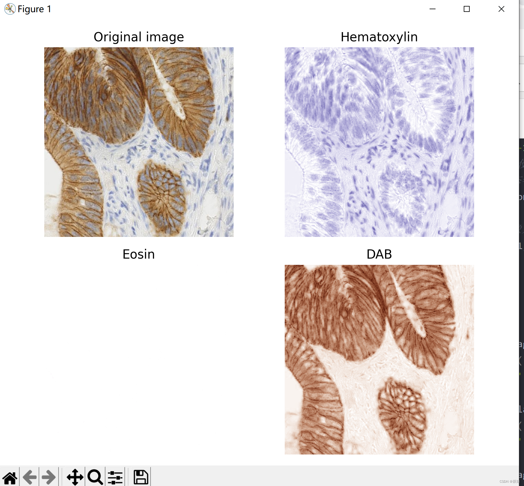
In this case , We will immunohistochemical staining (IHC) Anti staining separation with hematoxylin . Separation is used 1 The method described in , be called “ Color deconvolution ”.
Immunohistochemical staining showed , Diaminobenzidine (DAB) Show FHL2 The expression of protein is brown .
Color space 、hed Color channel concept :https://www.cnblogs.com/fydeblog/p/9737261.html
import numpy as np
import matplotlib.pyplot as plt

from skimage import data
from skimage.color import rgb2hed, hed2rgb

#  Get photo
ihc_rgb = data.immunohistochemistry()

#  Separate stains from immunohistochemical images
#RGB To Haematoxylin-Eosin-DAB (HED)  Color space conversion .
ihc_hed = rgb2hed(ihc_rgb)

#  Create one for each stain RGB Images
#np.zeros_like(a) The purpose of is to build a relationship with a Arrays of the same dimension , And initialize all variables to zero .
null = np.zeros_like(ihc_hed[:, :, 0])# Is to take all the data of the first dimension in the three-dimensional matrix , And the assignment is 0
ihc_h = hed2rgb(np.stack((ihc_hed[:, :, 0], null, null), axis=-1))# Su Mu is exquisite  RGB  Color space conversion ,axis=-1: In the last dimension , And convert to rgb
hed2rgb(np.stack((null, ihc_hed[:, :, 1], null), axis=-1))# Yi Hong arrives  RGB  Color space conversion
ihc_d = hed2rgb(np.stack((null, null, ihc_hed[:, :, 2]), axis=-1))#DAB (HED)  To  RGB  The transformation of color space

#  Exhibition
fig, axes = plt.subplots(2, 2, figsize=(7, 6), sharex=True, sharey=True)
ax = axes.ravel()
# Original picture
ax[0].imshow(ihc_rgb)
ax[0].set_title("Original image")
# Hematoxylin
ax[1].imshow(ihc_h)
ax[1].set_title("Hematoxylin")
# Yi Hong
ax[2].imshow(ihc_e)
ax[2].set_title("Eosin")  # Note that there is no Eosin stain in this image
#D passageway
ax[3].imshow(ihc_d)
ax[3].set_title("DAB")

for a in ax.ravel():
    a.axis('off')

fig.tight_layout()

# Now we can easily operate hematoxylin and DAB passageway :
from skimage.exposure import rescale_intensity

#  take h and d Brightness level of the channel rescale To (0,1)
# Re measure hematoxylin and DAB Channels and give them fluorescence observation , Adjust the image intensity according to a certain proportion
h = rescale_intensity(ihc_hed[:, :, 0], out_range=(0, 1),
                      in_range=(0, np.percentile(ihc_hed[:, :, 0], 99)))
d = rescale_intensity(ihc_hed[:, :, 2], out_range=(0, 1),
                      in_range=(0, np.percentile(ihc_hed[:, :, 2], 99)))
'''  Adjust the intensity   function :skimage.exposure.rescale_intensity(image, in_range='image', out_range='dtype') in_range: Indicates the intensity range of the input picture , The default is 'image',  Represents the maximum size of the image / The minimum pixel value is used as the range  out_range: Indicates the intensity range of the output picture , The default is 'dype',  Represents the maximum of the type of image used / The minimum value is used as the range   By default , Enter the name of the picture [min,max] The range is stretched to [dtype.min, dtype.max], If dtype=uint8,  that dtype.min=0, dtype.max=255 '''
# Render the two channels as RGB Images , Blue and green channels
# Add the two channels
zdh = np.dstack((null, d, h))# Why do you do this
#np.dstack Detailed explanation :https://www.cjavapy.com/article/894/
fig = plt.figure()
axis = plt.subplot(1, 1, 1, sharex=ax[0], sharey=ax[0])
axis.imshow(zdh)
axis.set_title('Stain-separated image (rescaled)')
axis.axis('off')
plt.show()

3、 Maximum value of filter area
ad locum , We use morphological reconstruction to create a background image , We can subtract it from the original image to separate bright features ( Area maximum ).
First , We start from the edge of the image , Try to rebuild through expansion . We initialize the seed image to the minimum intensity of the image ,
And set its boundary to the pixel value in the original image . These largest pixels will be enlarged to reconstruct the background image .
import skimage
''' Create a background image by morphological reconstruction , Subtract the background image from the original image to enhance the foreground . Morphological reconstruction involves two images and a structural element , An image is a mark ( That is what we will use next seed), It contains the starting point of the transformation , Another image is a template (mask), It is used to constrain the transformation . '''
import numpy as np
import matplotlib.pyplot as plt
from scipy.ndimage import gaussian_filter
from skimage import data
from skimage import img_as_float
from skimage.morphology import reconstruction
# Convert to floating point : This is important for the following subtraction , But not for uint8
#image = img_as_float(data.coins())# Transformation format
image=img_as_float(skimage.io.imread('11.jpg',))
image = gaussian_filter(image, 1)# Gauss filter is a linear smoothing filter , Gaussian noise can be removed , Its effect is to reduce sharp changes in image gray , That is, the image is blurred
''' def gaussian_filter(input, sigma, order=0, output=None, mode="reflect", cval=0.0, truncate=4.0): Input parameters : input: Input to the function is the matrix sigma: Scalar or scalar sequence , It's the Gaussian function \sigma, The bigger this is , The more blurred the filtered image Return value : The return value is the same matrix as the input shape '''
# Seed image initializes the minimum value of the image , And set its boundary to the pixel value of the original image
seed = np.copy(image)
seed[1:-1, 1:-1] = image.min()
mask = image# Use the original drawing as mask
# Morphological reconstruction with dilation
dilated = reconstruction(seed, mask, method='dilation')
# After subtracting the inflated image, only coins and a flat black background are left , As shown in the figure below .
fig, (ax0, ax1, ax2) = plt.subplots(nrows=1,
ncols=3,
figsize=(8, 2.5),
sharex=True,
sharey=True)
ax0.imshow(image, cmap='gray')
ax0.set_title('original image')
ax0.axis('off')
ax1.imshow(dilated, vmin=image.min(), vmax=image.max(), cmap='gray')
ax1.set_title('dilated')
ax1.axis('off')
ax2.imshow(image - dilated, cmap='gray')
ax2.set_title('image - dilated')
ax2.axis('off')
fig.tight_layout()
''' Although the characteristics ( The coin ) Is obviously isolated , But coins surrounded by a bright background in the original image are dimmer in the subtracted image . We can try to use different seed images to correct this problem . We can use the characteristics of the image itself to seed the reconstruction process , Instead of creating a seed image with a maximum value on the image boundary . here , The seed image is the original image minus a fixed value h '''
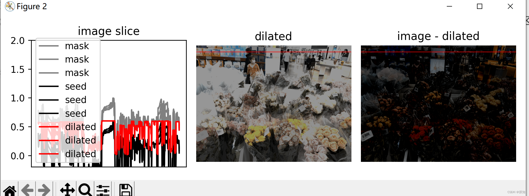
# Use the characteristics of the image itself as the basis of the reconstruction process seed, This time seed Set to subtract a fixed value from the original image h.
h = 0.4
seed = image - h
dilated = reconstruction(seed, mask, method='dilation')
hdome = image - dilated
# In order to get the feeling of the reconstruction process , We follow a slice of the image ( Denoted by a red line ) Draw mask 、 The intensity of seeds and enlarged images .
fig, (ax0, ax1, ax2) = plt.subplots(nrows=1, ncols=3, figsize=(8, 2.5))
yslice = 100
ax0.plot(mask[yslice], '0.5', label='mask')
ax0.plot(seed[yslice], 'k', label='seed')
ax0.plot(dilated[yslice], 'r', label='dilated')
ax0.set_ylim(-0.2, 2)
ax0.set_title('image slice')
ax0.set_xticks([])
ax0.legend()
ax1.imshow(dilated, vmin=image.min(), vmax=image.max(), cmap='gray')
ax1.axhline(yslice, color='r', alpha=0.4)
ax1.set_title('dilated')
ax1.axis('off')
ax2.imshow(hdome, cmap='gray')
ax2.axhline(yslice, color='r', alpha=0.4)
ax2.set_title('image - dilated')
ax2.axis('off')
''' The functionality : Draw parallel to x Horizontal reference line of axis Call signature :plt.axhline(y=0.0, c="r", ls="--", lw=2) y: The starting point of the horizontal reference line c: The line color of the reference line ls: The line style of the reference line lw: The line width of the reference line '''
fig.tight_layout()
plt.show()
As you can see in the image slice , Each coin is given a different baseline intensity in the reconstructed image ;
This is because we use local strength ( The offset h) As a seed value . therefore , The coins in the subtracted image have similar pixel intensity .
The final result is called image h-dome, Because this tends to isolate the height h Area maximum of . When your image is illuminated unevenly , This operation is particularly useful .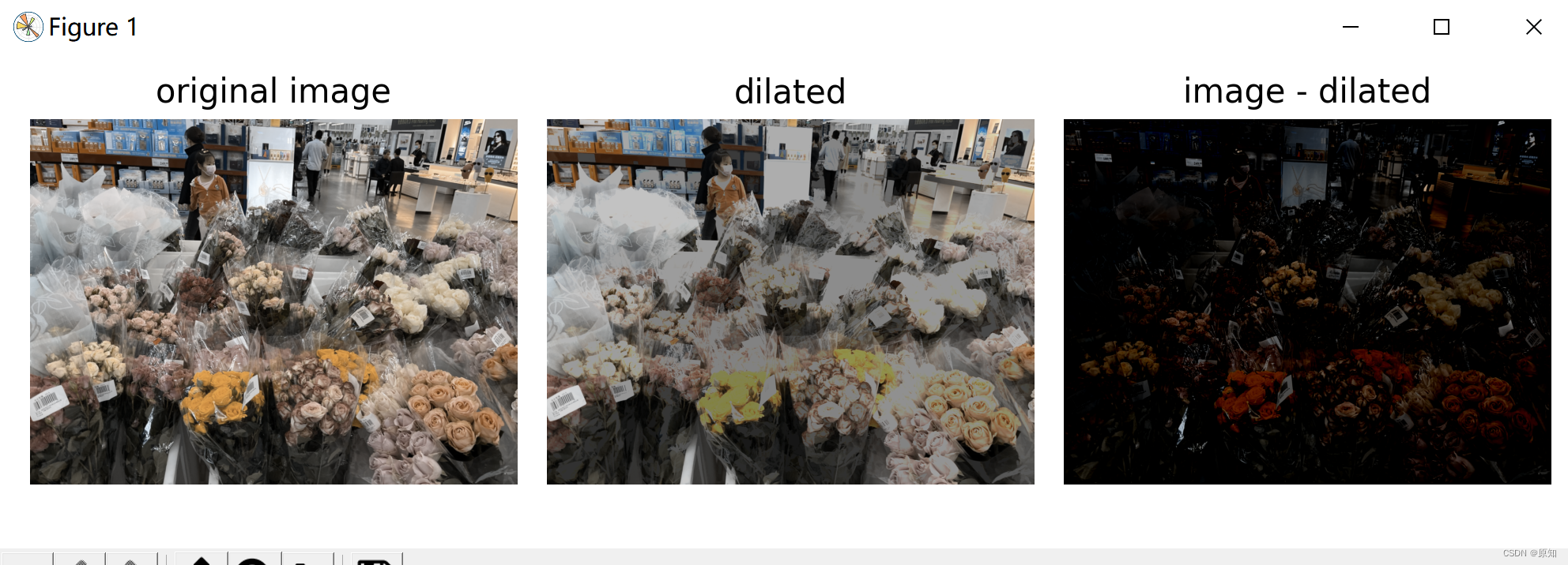
边栏推荐
猜你喜欢

随机推荐
【PHP】PHP接口继承及接口多继承原理与实现方法
Prediction - Grey Prediction
[medical segmentation] attention Unet
QT中自定义控件的创建到封装到工具栏过程(一):自定义控件的创建
LeetCode 1049. 最后一块石头的重量 II 每日一题
最新阿里P7技术体系,妈妈再也不用担心我找工作了
QML beginner
LeetCode 1774. The dessert cost closest to the target price is one question per day
LeetCode 1155. 掷骰子的N种方法 每日一题
面向接口编程
ByteDance Android gold, silver and four analysis, Android interview question app
typescript ts 基础知识之类型声明
QT picture background color pixel processing method
LeetCode 300. 最长递增子序列 每日一题
低代码(lowcode)帮助运输公司增强供应链管理的4种方式
Personal notes of graphics (2)
Have fun | latest progress of "spacecraft program" activities
二叉搜索树(特性篇)
Personal notes of graphics (4)
第九届 蓝桥杯 决赛 交换次数