当前位置:网站首页>Automatically generate VGg image annotation file
Automatically generate VGg image annotation file
2022-07-02 19:41:00 【woshicver】

In the field of computer vision , Instance segmentation is one of the hottest topics nowadays .
It includes the detection of objects in the image / Division , That is, the location of a specific object and the association of its pixels . Like any machine learning system , Training the backbone structure requires a large number of images . More specifically , A large number of annotations are needed to train the positioning function of neural network .
Annotation is a time-consuming activity , Can decide whether the project will succeed . therefore , Care must be taken , To increase productivity .
In the field of satellite images , Free data sets can be used to take advantage of previous work done by researchers or commentators . These datasets are usually built by researchers from open source images 、 It is released after pre-processing and post-processing and used to train and test their own artificial intelligence research system .
Semantic segmentation is a little different from instance segmentation , But in the case of buildings , One can help another .
in fact , Buildings are usually unique , It can be separated on any image . Take advantage of this consideration , A separate mask can be generated for each building from the binary label image , Then it is used to train the instance segmentation algorithm faster , Such as Mask RCNN. Comments do not have to be executed manually , This is the main advantage of this technology . Here are some tips on how to do it !
JSON File format
Mask RCNN Matterport Realize and FAIR Detectron2 Platform use JSON File loads comments for the training image data set . This file format is used in many computer science applications , Because it allows alphanumeric information to be easily stored and shared in the format of paired attribute values .
It is for JavaScript language-constructed , But now , It is used in many other programming languages , Such as Python. Special libraries have been established , In the Python The code is generated and parsed in the form of text files JSON Formatted data .VGG Annotation tool format Mask RCNN Typical used JSON The file will have the following shape :
{
  "image1.png9259408": {
    "filename": "image1.png",
    "size": 9259408,
    "regions": [
      {
        "shape_attributes": {
          "name": "polygon",
          "all_points_x": [
            314,
            55,
            71,
            303,
            318,
            538,
          ],
          "all_points_y": [
            1097,
            1093,
            1450,
            1450,
            1505,
            1474,
          ]
        },
        "region_attributes": {
          "class": "building"
        }
      },
      {
        "shape_attributes": {
          "name": "rect",
          "x": 515,
          "y": 1808,
          "width": 578,
          "height": 185
        },
        "region_attributes": {
          "class": "apple"
        }
      }
    ],
    "file_attributes": {}
  },
  "0030fd0e6378.png236322": {
    "filename": "0030fd0e6378.png",
    "size": 236322,
    "regions": [
      {
        "shape_attributes": {
          "name": "polygon",
          "all_points_x": [
            122,
            294,
            258,
            67,
            32
          ],
          "all_points_y": [
            92,
            113,
            231,
            221,
            132
          ]
        },
        "region_attributes": {
          "class": "apple"
        }
      },
      {
        "shape_attributes": {
          "name": "circle",
          "cx": 210,
          "cy": 303,
          "r": 47
        },
        "region_attributes": {
          "class": "swan"
        }
      }
    ],
    "file_attributes": {}
  }
}
One JSON Annotation files collect all annotation data . Each image annotation is stacked in a large JSON In file .
An image is identified by its identifier . The identifier is described by four attributes : The name of the image ( file name )、 Its size on disk ( size )、 The shape of the note ( Area ) And some metadata on the image ( File attribute ).
Each annotation can be described by two elements : Shape description ( Shape properties ) And annotation data ( Area properties ). The shape attribute describes the shape of the annotation ( name ) And an ordered list of two integers ( All points x And all points y) form , They represent the points that make up the mask annotation x and y coordinate . Annotation data region_attributes You can adjust , Annotation classes can be saved for multi class segmentation .
The fourth identifier attribute is named file_attributes, It can be used to store any information on the annotation image .
In grammar , Let's notice the braces {} Usually used to separate elements of the same type , And reference the attributes that describe an element . square brackets [] Used to represent the parameter list .
Fortunately, ,Python There is a library for us to read and write JSON file . Use import json Code snippets can easily load it , To read and write text files .
In the next chapter , We will discuss how to convert binary label images to VGG notes , Especially how to use JSON Syntax writing annotation file .
Generate annotations JSON file
The main idea of this paper is to convert binary label image into VGG Mask of annotation format JSON file . Personalize each shape of the binary label image , To convert it into a mask element , For example, segmentation .
The transformation mainly uses the famous OpenCV Graphics library execution , The library is located in Python Easy to use in .
def Annot(preprocess_path, res=0.6, surf=100, eps=0.01):
  """
  preprocess_path : path to folder with gt and images subfolder containing ground truth binary label image and visual imagery
  res : spatial resolution of images in meter
  surf : the minimum surface of roof considered in the study in square meter
  eps : the index for Ramer–Douglas–Peucker (RDP) algorithm for contours approx to decrease nb of points describing a contours
  """

    jsonf = {} # only one big annotation file
    with open(os.path.join(preprocess_path,'via_region_data.json'), 'w') as js_file:
        gt_path = os.path.join(preprocess_path, 'gt')
        images_path = os.path.join(preprocess_path, 'images')

        # All the elements in the images folders
        lst = os.listdir(images_path)
        for elt in tqdm(lst, desc='lst'):

            # Read the binary mask, and find the contours associated
            gray = cv2.imread(os.path.join(gt_path, elt))
            imgray = cv2.cvtColor(gray, cv2.COLOR_BGR2GRAY)
            _, thresh = cv2.threshold(imgray, 127, 255, 0)
            contours, _ = cv2.findContours(thresh, cv2.RETR_TREE, cv2.CHAIN_APPROX_SIMPLE)

            # https://www.pyimagesearch.com/2021/10/06/opencv-contour-approximation/
            # Contours approximation based on Ramer–Douglas–Peucker (RDP) algorithm
            areas = [cv2.contourArea(contours[idx])*res*res for idx in range(len(contours))]
            large_contour = []
            for i in range(len(areas)):
                if areas[i]>surf:
                    large_contour.append(contours[i])
            approx_contour = [cv2.approxPolyDP(c, eps * cv2.arcLength(c, True), True) for c in large_contour]

            # -------------------------------------------------------------------------------
            # BUILDING VGG ANNTOTATION TOOL ANNOTATIONS LIKE
            if len(approx_contour) > 0:
                regions = [0 for i in range(len(approx_contour))]
                for i in range(len(approx_contour)):
                    shape_attributes = {}
                    region_attributes = {}
                    region_attributes['class'] = 'roof'
                    regionsi = {}
                    shape_attributes['name'] = 'polygon'
                    shape_attributes['all_points_x'] = approx_contour[i][:, 0][:, 0].tolist()
                    # https://stackoverflow.com/questions/26646362/numpy-array-is-not-json-serializable
                    shape_attributes['all_points_y'] = approx_contour[i][:, 0][:, 1].tolist()
                    regionsi['shape_attributes'] = shape_attributes
                    regionsi['region_attributes'] = region_attributes
                    regions[i] = regionsi

                size = os.path.getsize(os.path.join(images_path, elt))
                name = elt + str(size)
                json_elt = {}
                json_elt['filename'] = elt
                json_elt['size'] = str(size)
                json_elt['regions'] = regions
                json_elt['file_attributes'] = {}
                jsonf[name] = json_elt

        json.dump(jsonf, js_file)
The first line is to build the correct folder path for real tags and image folders , And create JSON File Comments .
First , Use cv2.findContours Cut the binary mask into contours . Most conversions ( threshold 、 Gray scale conversion ) It doesn't really need to be , Because the data is already a binary image .cv2.findContours Function provides a list of contour lines , As a list of points , The coordinates of these points are represented in the reference system of the image .
In large building roof projects , Can use custom OpenCV Function to export the roof surface , Then convert it into square meters , And only select roofs with sufficient area . under these circumstances , have access to Ramer–Douglas–Peucker(RDP) Algorithm to simplify and approximate the detected contour , In order to store annotation data more compactly . here , You should have a list of points , These points represent the contour detected on the binary image .
Now? , You need to convert the whole contour point list into a large one for mask RCNN Algorithm via_region_data.json file . about JSON notes , The data needs to have the format specified in the first paragraph . Dictionaries mainly push data to JSON Use before file .
According to the outline [] The number of , A specific number of [:,0] To get the correct data . An array of integers describing the outline must be converted to JSON Serializable data . Make VGG notes JSON The file is very similar to making Russian dolls . You can create an empty dictionary , Specify one ( Or more ) The value of the property , Then pass it as the value of a higher-level attribute , To encapsulate it into a larger dictionary . We noticed that , For multi class segmentation or object detection ,region_attributes It can contain an attribute class , The mask of this attribute class is shape_attributes Specified in parameter .
Last , Put all image data into JSON Documents before , Each image data is stored in a large “json” In the elements , Its name + Size string as identifier . This is very important , Because if you write every time you run a new image JSON file ,JSON Mask of file RCNN Import will fail . This is because json.load Read only the first set of braces {} The content of , Unable to explain the next set of braces .
That's it ! Let's see what the result of this process is !
Check the comment display
This small chapter will show the graphical use of the above process . It mainly uses the images of American cities publicly released by the U.S. Geological Survey through the national map service ( Chicago 、 Austin 、 San Francisco ).
Map services and data provided by the National Geospatial program of the United States Geological Survey . The service is open source , So you can do whatever you want with the data !
In this article , Processed high-resolution images near Austin, Texas ( Spatial resolution =0.3 rice / Pixels ).
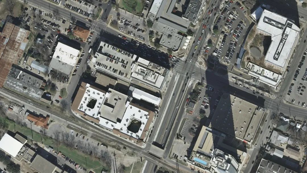
The first image is a visual color image , Usually, the GeoTiff Format provided , It also contains embedded geospatial data . It features the urban scene of the American urban environment . Rendering is constructed from three spectral visual images : Usual blue 、 Green and red . But in more complex images , Image suppliers can provide near infrared images , In order to be able to generate CNIR( colour + Near infrared images ), To analyze different aspects of spectral images .
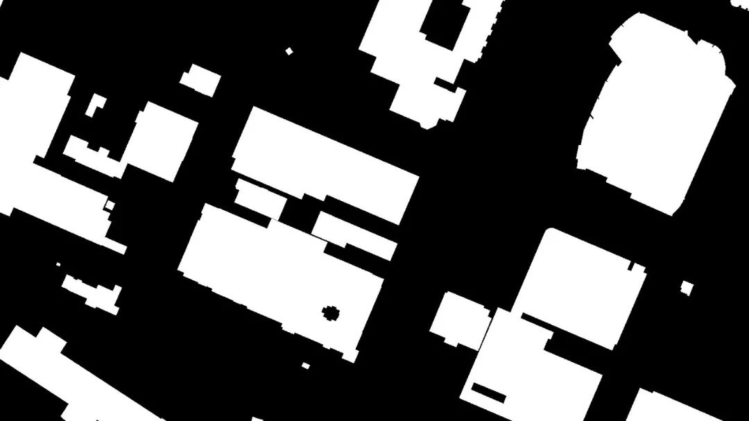
The second image shows the binary label image . It can be seen that , The label contains every pixel related to the building , Even the smallest curved pixels . Each building can be identified individually , Because buildings cannot overlap , This proves the rationality of the whole process .
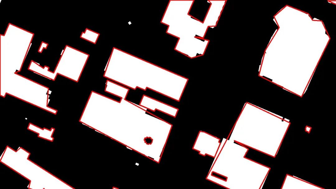
The third image consists of binary labels 1 and cv2 The detected contour composition , Highlighted in red . The contour lines displayed are from OpenCV Raw data of function , Not filtered out , So even the smallest building will be shown . It should be noted that ,cv2.findContours It is a pixel level conversion : The two buildings connected by a pixel will be divided together , Only one row of dark pixels is enough to separate two adjacent buildings .

The fourth image shows a binary label image with a filtered approximate contour . As the second chapter says , For the roof project , For areas less than 100 Square meters of buildings are not interested . It will also perform contour approximation to reduce the size of the annotation file . therefore , Outline only around large buildings , In some cases , The outline does not exactly match the shape of the building , Cannot inspire contour approximation .
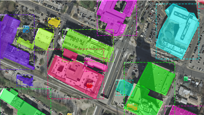
The fifth and last image shows the usual example segmentation visualization , have access to inspect_roof_data And other tools . The roof of a large building is divided separately .
Conclusion
The process shown in this article shows how to transform semantic data sets into instance segmentation training data sets . Then you can use it to train effectively Mask-RCNN Algorithm . This process can also be reused and modified , To accommodate datasets with different input label shapes .
* END *
If you see this , Show that you like this article , Please forward 、 give the thumbs-up . WeChat search 「uncle_pn」, Welcome to add Xiaobian wechat 「 woshicver」, Update a high-quality blog post in your circle of friends every day .
↓ Scan QR code and add small code ↓

边栏推荐
- PHP asymmetric encryption method private key and public key encryption and decryption method
- AcWing 1128. 信使 题解(最短路—Floyd)
- AcWing 343. Sorting problem solution (Floyd property realizes transitive closure)
- AcWing 181. 回转游戏 题解(搜索—IDA*搜索)
- VBScript详解(一)
- Py之interpret:interpret的简介、安装、案例应用之详细攻略
- 450-深信服面经1
- AcWing 1127. 香甜的黄油 题解(最短路—spfa)
- AcWing 181. Turnaround game solution (search ida* search)
- Yes, that's it!
猜你喜欢

Zabbix5 client installation and configuration

SQLite 3.39.0 release supports right external connection and all external connection

End to end object detection with transformers (Detr) paper reading and understanding
Reading notes of "the way to clean structure" (Part 2)

IEDA refactor的用法

编写完10万行代码,我发了篇长文吐槽Rust
How to avoid duplicate data in gaobingfa?
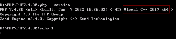
Windows2008R2 安装 PHP7.4.30 必须 LocalSystem 启动应用程序池 不然500错误 FastCGI 进程意外退出

rxjs Observable 自定义 Operator 的开发技巧

《重构:改善既有代码的设计》读书笔记(上)
随机推荐
股票证券公司排名,有安全保障吗
Microservice technology - distributed global ID in high concurrency
Web2.0 giants have deployed VC, and tiger Dao VC may become a shortcut to Web3
《代碼整潔之道》讀書筆記
高并发下如何避免产生重复数据?
Data dimensionality reduction factor analysis
452-strcpy、strcat、strcmp、strstr、strchr的实现
4274. 后缀表达式-二叉表达式树
Build a master-slave mode cluster redis
Dictionaries
mysql函数
AcWing 383. Sightseeing problem solution (shortest circuit)
Codeworks round 802 (Div. 2) pure supplementary questions
Refactoring: improving the design of existing code (Part 1)
453-atoi函数的实现
MySQL advanced (Advanced) SQL statement
Introduction to mongodb chapter 03 basic concepts of mongodb
AcWing 1128. 信使 题解(最短路—Floyd)
Golang:[]byte to string
Chapter 7 - class foundation