当前位置:网站首页>[video memory optimization] deep learning video memory optimization method
[video memory optimization] deep learning video memory optimization method
2022-07-01 15:35:00 【Dudu is too delicious】
Deep learning gpu Video memory of is very important , If the video memory is too small , The model can't run at all , This paper introduces several optimization methods when the video memory is insufficient , It can reduce the video memory requirements of the deep learning model .
Catalog
One 、 Gradient accumulation
Gradient accumulation refers to the process of model training , Train one batch After getting the gradient of the data , Do not immediately update the model parameters with this gradient , Instead, go on to the next batch Data training , Get the gradient and continue the cycle , After many cycles, the gradient keeps accumulating , Until a certain number of times , Update parameters with accumulated gradients , This can play a disguised expansion batch_size The role of .
model = SimpleNet()
mse = MSELoss()
optimizer = SGD(params=model.parameters(), lr=0.1, momentum=0.9)

accumulate_batchs_num = 10 #  Add up 10 Sub gradient

for epoch in range(epochs):
    for i, (data, label) in enumerate(loader):

        output = model(data)
        loss = mse(output, label)

        scaled.backward()
        #  When the cumulative  batch  by  accumulate_batchs_num  when , Update model parameters
        if (i + 1) % accumulate_batchs_num == 0:
            #  Training models
            optimizer.step()
            optimizer.clear_grad()
Two 、 Mixing accuracy
Reference resources : Mixed precision training
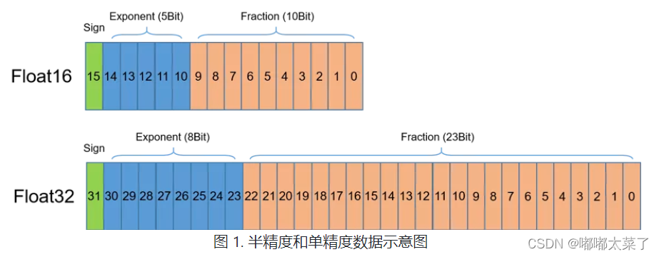
Floating point data types are mainly divided into double precision (FP64)、 Single precision (FP32)、 Semi precision (FP16), As shown in the figure , Semi precision (FP16) Is a relatively new floating point type , To use in a computer 2 byte (16 position ) Storage . stay IEEE 754-2008 In the standard , It is also called binary16. And the single precision commonly used in calculation (FP32) Double precision (FP64) Type comparison ,FP16 It is more suitable for use in scenes with low accuracy requirements .
With the same super parameters , Mixed precision training uses half precision floating point (FP16) And single precision (FP32) Floating point can achieve the same accuracy as pure single precision training , And it can accelerate the training speed of the model , This is mainly due to NVIDIA from Volta Architecture began to roll out Tensor Core technology . In the use of FP16 The calculation has the following characteristics :
FP16 It can reduce memory bandwidth and storage requirements by half , This allows researchers to use larger and more complex models and larger batch size size .
FP16 You can make full use of NVIDIA Volta、Turing、Ampere framework GPU Provided Tensor Cores technology . In the same GPU On the hardware ,Tensor Cores Of FP16 The calculated throughput is FP32 Of 8 times .
But use FP16 There will also be the following shortcomings :
- Data overflow : Data overflow is easy to understand ,FP16 comparison FP32 The effective range of is much narrower , Use FP16 Replace FP32 There will be an overflow (Overflow) And underflow (Underflow) The situation of . And in deep learning , The gradient of weight in the network model needs to be calculated ( First derivative ), Therefore, the gradient will be smaller than the weight value , Often prone to underflow .
- Rounding error :Rounding Error The indication is when the reverse gradient of the network model is very small , commonly FP32 Be able to express , But switch to FP16 Will be less than the minimum interval in the current interval , Can cause data overflow . Such as 0.00006666666 stay FP32 Can normally express , The switch to FP16 It will be expressed as 0.000067, dissatisfaction FP16 The number of minimum intervals is forcibly rounded .
For deep learning training, you can use FP16 The benefits of , Also avoid precision overflow and rounding error . So you can go through FP16 and FP32 Mixed precision training for (Mixed-Precision), Weight backup can be introduced in the process of mixed accuracy training (Weight Backup)、 Loss amplification (Loss Scaling)、 Precision accumulation (Precision Accumulated) Three related technologies .
1、 Weight backup
Weight backup is mainly used to solve the problem of rounding error . The main idea is to integrate the activation generated in the process of neural network training activations、 gradient gradients、 Intermediate variables and other data , Use... In training FP16 To store , Make a copy at the same time FP32 Weight parameter of weights, For training updates . The details are shown in the following figure , In forward and reverse calculations , Use FP16, But update parameters using FP32.

2、 Loss scaling
In the process of network back propagation , The value of the gradient is usually very small , If you use FP32 Can train normally , But if you use FP16, because FP16 The scope of expression ( The part on the left of the red line in the figure below is FP16 All of them are for 0), It will result in a smaller gradient of 0, The parameters cannot be optimized , The model doesn't converge .

In order to solve the problem of data underflow with too small gradient , Scale the loss function , And then scale the parameters back when optimizing the parameters . The specific operation is :
① Forward propagation :loss = loss * s
② Back propagation :grad = grad / s
Multiply the loss function by a coefficient s, Then the gradient increases in equal proportion , When re optimizing parameters, scale them to 1/s, Then the problem of gradient value underflow can be solved .
torch The sample code is as follows , Reference resources :
# Creates model and optimizer in default precision
model = Net().cuda()
optimizer = optim.SGD(model.parameters(), ...)

# Creates a GradScaler once at the beginning of training.
scaler = GradScaler()

for epoch in epochs:
    for input, target in data:
        optimizer.zero_grad()

        # Runs the forward pass with autocasting.
        with autocast():
            output = model(input)
            loss = loss_fn(output, target)

        # Scales loss.  Calls backward() on scaled loss to create scaled gradients.
        # Backward passes under autocast are not recommended.
        # Backward ops run in the same dtype autocast chose for corresponding forward ops.
        scaler.scale(loss).backward()

        # scaler.step() first unscales the gradients of the optimizer's assigned params.
        # If these gradients do not contain infs or NaNs, optimizer.step() is then called,
        # otherwise, optimizer.step() is skipped.
        scaler.step(optimizer)

        # Updates the scale for next iteration.
        scaler.update()
3、 Precision accumulation
In the process of model training with mixed accuracy , Use FP16 Do matrix multiplication , utilize FP32 To accumulate in the middle of matrix multiplication (accumulated), And then FP32 The value of is converted to FP16 For storage . Briefly , Is the use FP16 Do matrix multiplication , utilize FP32 To make up for the lost accuracy . This can effectively reduce the rounding error in the calculation process , Minimize the loss of accuracy .
3、 ... and 、 Recalculation
Generally speaking, a training of deep learning network consists of three parts :
Forward calculation (forward): At this stage, the operator of the model will be forward calculated , Calculate the input of the operator to get the output , And send it to the next layer as input , Until the result position of the last layer is calculated ( Usually loss ).
Reverse calculation (backward): In this phase , The gradient of parameters of each layer will be calculated by reverse derivation and chain rule .
Gradient update ( Optimize ,optimization): In this phase , The parameters are updated by the gradient obtained by reverse calculation , Also called learning , Parameter optimization .
In the back propagation chain conduction , It needs the output of the middle layer to calculate the gradient of parameters , Therefore, the output of the middle layer will be saved in the training stage . In order to reduce the consumption of video memory , You can not save the calculation results of the m-server , When calculating gradient in back propagation , Then calculate the output of the middle layer by local forward , To calculate the gradient .
Recalculation is the operation of changing space through time .
边栏推荐
猜你喜欢

【目标跟踪】|STARK

Wechat applet 01 bottom navigation bar settings
![[STM32 learning] w25qxx automatic judgment capacity detection based on STM32 USB storage device](/img/41/be7a295d869727e16528041ad08cd4.png)
[STM32 learning] w25qxx automatic judgment capacity detection based on STM32 USB storage device

MySQL 服务正在启动 MySQL 服务无法启动解决途径

Junda technology indoor air environment monitoring terminal PM2.5, temperature and humidity TVOC and other multi parameter monitoring

STM32F411 SPI2输出错误,PB15无脉冲调试记录【最后发现PB15与PB14短路】

Fix the failure of idea global search shortcut (ctrl+shift+f)
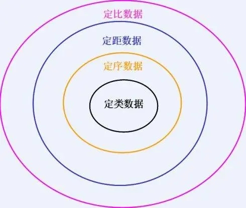
张驰课堂:六西格玛数据的几种类型与区别

Introduction to MySQL audit plug-in
《性能之巅第2版》阅读笔记(五)--file-system监测
随机推荐
OpenSSL client programming: SSL session failure caused by an insignificant function
常见健身器材EN ISO 20957认证标准有哪些
Skywalking 6.4 distributed link tracking usage notes
【OpenCV 例程200篇】216. 绘制多段线和多边形
[one day learning awk] function and user-defined function
[cloud trend] new wind direction in June! Cloud store hot list announced
[target tracking] | template update time context information (updatenet) "learning the model update for Siamese trackers"
Filter & (login interception)
SAP CRM organization Model(组织架构模型)自动决定的逻辑分析
Redis high availability principle
【天线】【3】CST一些快捷键
硬件开发笔记(九): 硬件开发基本流程,制作一个USB转RS232的模块(八):创建asm1117-3.3V封装库并关联原理图元器件
摩根大通期货开户安全吗?摩根大通期货公司开户方法是什么?
如何实现时钟信号分频?
SAP S/4HANA: 一条代码线,许多种选择
Don't ask me again why MySQL hasn't left the index? For these reasons, I'll tell you all
《QT+PCL第六章》点云配准icp系列5
A unifying review of deep and shallow anomaly detection
Opencv learning note 4 -- bank card number recognition
Flink 系例 之 TableAPI & SQL 与 MYSQL 插入数据