当前位置:网站首页>Detailed explanation of traditional image segmentation methods
Detailed explanation of traditional image segmentation methods
2022-06-26 08:46:00 【will be that man】
Catalog :
- 1. Overview of image segmentation algorithm
- 1.1 Threshold based segmentation method
- 1.2 Edge based segmentation method
- 1.3 Region based segmentation method
- 1.4 Segmentation method based on graph theory
- 1.5 Partition method based on energy functional
- 1.6 Image segmentation method based on wavelet analysis and wavelet transform
- 1.7 Image segmentation based on genetic algorithm
- 2. Threshold segmentation of image segmentation
- 3. Edge based segmentation method
- 4. Watershed algorithm for image segmentation
- 5. Image segmentation Mean shift Algorithm
Reprint :
- Adaptive threshold (adaptiveThreshold) Segmentation principle and implementation
- Section 8 、 Image segmentation GrabCut Algorithm 、 Watershed algorithm
- Otsu Algorithm
- Mean-Shift Algorithm
- mean shift Image segmentation ( One )
The so-called image segmentation is based on the gray level 、 Color 、 Texture and shape divide the image into several non overlapping regions , And make these features show similarity in the same area , And there are obvious differences between different regions . Let's give an overview of the main image segmentation methods , Later, we will have a detailed understanding and study of individual methods .
1. Overview of image segmentation algorithm
1.1 Threshold based segmentation method
The basic idea of threshold method is to calculate one or more gray thresholds based on the gray characteristics of the image , The gray value of each pixel in the image is compared with the threshold value , Finally, the pixels are divided into appropriate categories according to the comparison results . therefore , The key step of this kind of method is to solve the optimal gray threshold according to a certain criterion function .
1.2 Edge based segmentation method
The so-called edge refers to the set of continuous pixels on the boundary line of two different regions in the image , It is the reflection of the discontinuity of image local features , It's grayscale 、 Color 、 The mutation of image characteristics such as texture . Usually , Edge based segmentation refers to edge detection based on gray value , It is established that the gray value at the edge will show stepped or Roof type A method based on the observation of change .
There are obvious differences in the gray values of the pixels on both sides of the step edge , The roof edge is at the turning point of gray value rising or falling . Based on this characteristic , You can use differential operators for edge detection , That is, the extreme value of the first derivative and the zero crossing point of the second derivative are used to determine the edge , Specific implementation can be completed by convolution of image and template .
1.3 Region based segmentation method
This kind of method is to divide the image into different regions according to the similarity criterion , It mainly includes Seed zone growing method 、 Regional division and consolidation and Watershed And so on .
The seed region growing method starts with a group of seed pixels representing different growing regions , Next, the eligible pixels in the neighborhood of the seed pixel are merged into the growing region represented by the seed pixel , And the newly added pixels are used as new seed pixels to continue the merging process , Until we can't find a new pixel that meets the criteria . The key of this method is to select appropriate initial seed pixels and reasonable growth criteria .
Regional division and consolidation (Gonzalez,2002) The basic idea of is to divide the image into several disjoint regions , Then divide or merge these regions according to relevant criteria to complete the segmentation task , This method is suitable for both gray image segmentation and texture image segmentation .
Watershed (Meyer,1990) It is a mathematical morphology segmentation method based on topological theory , The basic idea is to regard the image as a topologic landform in geodesy , The gray value of each pixel in the image represents the altitude of the point , Each local minimum and its influence area is called a catchment basin , The boundary of the catchment basin forms a watershed . The implementation of the algorithm can simulate the process of flood inundation , The lowest point of the image is first submerged , Then the water gradually flooded the whole valley . When the water level reaches a certain height, it will overflow , And then build a dam where the water overflows , Repeat this process until all the points in the whole image are submerged , At this time, a series of dikes were built to divide the basins . Watershed algorithm has a good response to weak edges , But the noise in the image will make the watershed algorithm produce the phenomenon of over segmentation .
1.4 Segmentation method based on graph theory
This kind of method combines the problem of image segmentation with that of graph Minimum cut (min cut) The problems are related . First, the image is mapped to a weighted undirected graph G=<V,E>, Every node in the graph N∈V For each pixel in the image , Every side ∈E Connecting a pair of adjacent pixels , The weight of the adjacent pixels is between the edges 、 Non negative similarity in color or texture . And a segmentation of the image s It's a clipping of a graph , Every area that's divided C∈S Corresponding to a subgraph in the graph . The best principle of segmentation is to keep the maximum similarity within the partitioned subgraph , The similarity between subgraphs is kept to the minimum . The essence of graph theory based segmentation is to remove specific edges , The graph is divided into several subgraphs to achieve segmentation . At present, the methods based on graph theory are GraphCut,GrabCut and Random Walk etc. .
1.5 Partition method based on energy functional
This kind of method mainly refers to the active contour model (active contour model) And the algorithm based on it , The basic idea is to use continuous curve to express the target edge , An energy functional is defined so that its independent variables include edge curves , Therefore, the partition process is transformed into the process of solving the minimum value of the energy functional , Generally, we can solve the Euler corresponding to the function (Euler.Lagrange) We can use the equation to realize , The curve position where the energy reaches the minimum is the contour of the target . According to the different forms of curve expression in the model , Active contour models can be divided into two categories : Parametric active contour model (parametric active contour model) And geometric active contour models (geometric active contour model).
Parametric active contour model is based on Lagrange frame , Express the curve directly in the parametric form of the curve , The most representative is by Kasset a1(1987) The proposed Snake Model . This kind of model has been successfully applied in the field of early biological image segmentation , However, it has some disadvantages, such as the segmentation result is greatly affected by the setting of initial contour, and it is difficult to deal with the change of curve topology , In addition, the energy functional only depends on the choice of curve parameters , It has nothing to do with the geometry of the object , This also limits its further application .
The curve motion process of geometric active contour model is based on the geometric measurement parameters of the curve rather than the expression parameters of the curve , So we can deal with the change of topology better , And it can solve the problem that parametric active contour model is difficult to solve . Level set (Level Set) Method (Osher,1988) The introduction of , It greatly promotes the development of geometric active contour model , Therefore, geometric active contour model can also be called level set method .
1.6 Image segmentation method based on wavelet analysis and wavelet transform
Wavelet transform is a widely used mathematical tool in recent years , It is also a necessary part of digital image processing , It has a high degree of localization in both the time domain and the frequency domain , It can unify time domain and frequency domain to study signals . Moreover, wavelet transform has multi-scale characteristics , Be able to analyze signals on different scales , So it has been applied in image segmentation .
Dyadic wavelet transform has the ability to detect local mutation of binary function , Therefore, it can be used as an image edge detection tool . The edge of the image appears at the local gray discontinuity of the image , Corresponding to the modulus maxima of dyadic wavelet transform . By detecting the modulus maxima of wavelet transform, it can be determined that the edge wavelet transform of image is located on each scale , The wavelet transform on each scale can provide certain edge information , Therefore, multi-scale edge detection can be carried out to get an ideal image edge .

The above figure and the left figure are the traditional threshold segmentation methods , The image on the right is the image segmentation using wavelet transform . It can be seen that the edge of the right image segmentation is more accurate and clear
in addition , The combination of wavelet and other methods to deal with image segmentation has also been widely studied , For example, a local adaptive threshold method is to Hilbert Combination of image scanning and wavelet , Thus, a continuous and smooth threshold curve is obtained .
1.7 Image segmentation based on genetic algorithm
Genetic algorithm (ga) (Genetic Algorithms, abbreviation GA) yes 1973 By American professor Holland Proposed , It is a randomized search algorithm that draws lessons from the natural selection and natural genetic mechanism of Biology . It is the application of Bionics in the field of mathematics . The basic idea is this , Simulate the evolution of biological populations controlled by some gene strings , The principle of this process is applied to the search algorithm , To improve the speed and quality of optimization . The search process of this algorithm does not directly act on variables , It is the individual encoded in the parameter set , This makes the genetic algorithm can be directly applied to structural objects ( Images ) To operate . The whole search process is iterating from one set of solutions to another , The method of dealing with multiple individuals in a group at the same time , It reduces the possibility of falling into the local optimal solution , And easy to parallelize . The search process uses the transition rules of probability to guide the search direction , Instead of using deterministic search rules , And there are no special requirements for the search space ( Such as connectivity 、 Convexity, etc ), Use only adaptive information , No other auxiliary information such as derivatives is required , A wide range of applications .
Genetic algorithm is good at global search , But the local search ability is insufficient , Therefore, genetic algorithm is often combined with other algorithms . The application of genetic algorithm to image processing mainly considers that genetic algorithm has the ability of fast and random search independent of the problem domain . Its search starts from the group , It has potential parallelism , You can compare multiple individuals at the same time , It can effectively accelerate the speed of image processing . But genetic algorithm also has its disadvantages : The design of the evaluation function used in the search 、 The selection of the initial population has certain dependence . If we can combine some heuristic algorithms to improve and make full use of the parallel mechanism of genetic algorithm , This is a research hotspot of genetic algorithm in image processing .
2. Threshold segmentation of image segmentation
2.1 OSTU Algorithm
Otsu Algorithm , Also known as the maximum interclass variance method ( Otsu algorithm ), Is a global threshold algorithm .
The reason why it is called the maximum interclass variance method is because , Image fixed threshold binarization with the threshold , Maximum variance between classes , It's based on the grayscale characteristics of the image , Divide the image into two parts: background and foreground , The segmentation with the largest variance among classes means the least probability of misclassification .

principle :
For the image I(x,y), prospects ( That's the goal ) Record the background and threshold of segmentation T, The proportion of pixels belonging to the foreground to the whole image is marked as ω0, Its average gray level μ0; The proportion of background pixels to the whole image is ω1, The average gray level is μ1. The total average gray level of the image is recorded as μ, The variance between classes is recorded as g.
Suppose the background of the image is dark , And the size of the image is M×N, The gray value of pixels in the image is less than the threshold T The number of pixels is recorded as N0, The pixel gray is greater than the threshold T The number of pixels is recorded as N1, Then there are :
(1) ω0=N0/ (M×N)
(2) ω1=N1/ (M×N)
(3) N0 + N1 = M×N
(4) ω0 + ω1 = 1
(5) μ = ω0 * μ0 + ω1 * μ1
(6) g = ω0 * (μ0 - μ)2 + ω1 * (μ1 - μ)2
Will type (5) Substituting (6), Get the equivalent formula :
(7) g = ω0 *ω1 * (μ0 - μ1)2
Using the ergodic method, the inter class variance is obtained g Maximum threshold T.
Algorithm evaluation :
advantage : Method is simple , When there is little difference between the area of the target and the background , It can segment the image effectively .
shortcoming : When the area between the target and the background in the image is very different , There is no obvious bimodal in histogram , Or the two peaks are quite different in size , The segmentation effect is not good , Or when the gray level of the target and the background has a large overlap, it can not accurately separate the target and the background .
reason : This method ignores the spatial information of the image , At the same time, the gray distribution of the image is used as the basis of image segmentation , It is also quite sensitive to noise .
OpenCV Provided API:
double threshold(InputArray src, OutputArray dst, double thresh, double maxval, int type)
Parameters :
- src: Input diagram , Only single channel can be entered ,8 Bit or 32 Bit floating point number image .
- dst: Output chart , Size 、 The depth will be the same as the input map .
- thresh: threshold .
- maxval: The maximum value of the binarization result .
- type: Binary operation mode , share THRESH_BINARY、THRESH_BINARY_INV、THRESH_TRUNC、THRESH_TOZERO、THRESH_TOZERO_INV Five kinds .type From the above five combinations CV_THRESH_OTSU Namely OSTU Algorithm , It's written in :THRESH_BINARY | CV_THRESH_OTSU.
2.1.1 be based on OpenCV Realization
#include <cstdio>
#include <opencv2/opencv.hpp>

int main() {

    cv::Mat src = cv::imread("D:\\code\\C++\\ Image segmentation \\image segmentation\\test_pic\\OSTU\\car.png");
    if (src.empty()) {

        return -1;
    }
    if (src.channels() > 1)
        cv::cvtColor(src, src, cv::COLOR_RGB2GRAY);

    cv::Mat dst;
    threshold(src, dst, 0, 255, cv::THRESH_BINARY | cv::THRESH_OTSU); //  Because it is OSTU Algorithm ,threshold This parameter is useless

    cv::namedWindow("src", cv::WINDOW_NORMAL);
    cv::imshow("src", src);
    cv::namedWindow("dst", cv::WINDOW_NORMAL);
    cv::imshow("dst", dst);
    cv::imwrite("D:\\code\\C++\\ Image segmentation \\image segmentation\\test_pic\\OSTU\\car_output.png", dst);
    cv::waitKey(0);

    return 0;
}
We tested a picture of an ordinary car , The results are shown below :

Now we're right kitti Image and speckle structured light image segmentation , The results are shown below :

- real-general

real-indoor1

real-indoor2

real-indoor3

real-outdoor

synthetic-intel

synthetic-ideal

synthetic-polka

2.2 Adaptive threshold method
Adaptive threshold method (adaptiveThreshold), Its idea is not to calculate the threshold value of the global image , It depends on the brightness distribution of different areas of the image , Calculate its local threshold , So for different areas of the image , Can adaptively calculate different thresholds , So it's called adaptive threshold method .( In fact, it's the local threshold method )
How to determine the local threshold ? You can calculate a neighborhood ( Local ) Of mean value 、 The median 、 Gauss weighted average ( Gauss filtering ) To determine the threshold . It's worth noting that : If we use the local mean as the local threshold , It's called moving average .
OpenCV Provided API:
void adaptiveThreshold(InputArray src, OutputArray dst, double maxValue,
                      int adaptiveMethod, int thresholdType, int blockSize, double C)
Parameters :
- InputArray src: The source image
- OutputArray dst: Output image , Consistent with the size of the source image
- int adaptiveMethod: The algorithm used to calculate the threshold in a neighborhood , There are two values , Respectively ADAPTIVE_THRESH_MEAN_C and ADAPTIVE_THRESH_GAUSSIAN_C .
- ADAPTIVE_THRESH_MEAN_C The calculation method is to calculate the average value of the field and subtract the seventh parameter double C Value .
- ADAPTIVE_THRESH_GAUSSIAN_C The calculation method is to calculate the Gaussian mean of the field and subtract the seventh parameter double C Value .
- int thresholdType: This is the threshold type , There are several options .
- THRESH_BINARY Binary thresholding -> Greater than the threshold is 1 Less than the threshold is 0
- THRESH_BINARY_INV Anti binary thresholding -> Greater than the threshold is 0 Less than the threshold is 1
- THRESH_TRUNC Truncation thresholding -> Greater than the threshold is the threshold , Less than the threshold does not change
- THRESH_TOZERO Threshold to 0 -> Constant greater than the threshold , All below the threshold are 0
- THRESH_TOZERO_INV Reverse thresholding to 0 -> Greater than the threshold is 0, Less than the threshold does not change
- int blockSize:adaptiveThreshold The unit of calculation is the neighborhood block of pixels , This is the local neighborhood size ,3、5、7 etc. .
- double C: This parameter is actually an offset adjustment , After calculating the threshold with mean and Gauss , Then subtract this value to get the final threshold .
notes : comparison OpenCV Of API, I used a median method to determine the threshold .
2.2.1 be based on OpenCV Realization
#include <iostream>
#include <opencv2/core.hpp>
#include <opencv2/highgui.hpp>
#include <opencv2/imgproc.hpp>


enum adaptiveMethod { meanFilter, gaaussianFilter, medianFilter };

void AdaptiveThreshold(cv::Mat& src, cv::Mat& dst, double Maxval, int Subsize, double c, adaptiveMethod method = meanFilter) {

	if (src.channels() > 1)
		cv::cvtColor(src, src, cv::COLOR_RGB2GRAY);

	cv::Mat smooth;
	switch (method)
	{
	case  meanFilter:
		cv::blur(src, smooth, cv::Size(Subsize, Subsize));  // Mean filtering
		break;
	case gaaussianFilter:
		cv::GaussianBlur(src, smooth, cv::Size(Subsize, Subsize), 0, 0); // Gauss filtering
		break;
	case medianFilter:
		cv::medianBlur(src, smooth, Subsize);   // median filtering
		break;
	default:
		break;
	}

	smooth = smooth - c;

	// Threshold processing
	src.copyTo(dst);
	for (int r = 0; r < src.rows; ++r) {
		const uchar* srcptr = src.ptr<uchar>(r);
		const uchar* smoothptr = smooth.ptr<uchar>(r);
		uchar* dstptr = dst.ptr<uchar>(r);
		for (int c = 0; c < src.cols; ++c) {
			if (srcptr[c] > smoothptr[c]) {
				dstptr[c] = Maxval;
			}
			else
				dstptr[c] = 0;
		}
	}

}

int main() {
	cv::Mat src = cv::imread("D:\\code\\C++\\ Image segmentation \\image segmentation\\test_pic\\car.png");
	if (src.empty()) {
		return -1;
	}
	if (src.channels() > 1)
		cv::cvtColor(src, src, cv::COLOR_RGB2GRAY);

	cv::Mat dst, dst2;
	double t2 = (double)cv::getTickCount();
	AdaptiveThreshold(src, dst, 255, 21, 10, meanFilter);  //
	t2 = (double)cv::getTickCount() - t2;
	double time2 = (t2 * 1000.) / ((double)cv::getTickFrequency());
	std::cout << "my_process=" << time2 << " ms. " << std::endl << std::endl;

	cv::adaptiveThreshold(src, dst2, 255, cv::ADAPTIVE_THRESH_MEAN_C, cv::THRESH_BINARY, 21, 10);

	cv::namedWindow("src", cv::WINDOW_NORMAL);
	cv::imshow("src", src);
	cv::namedWindow("dst", cv::WINDOW_NORMAL);
	cv::imshow("dst", dst);
	cv::namedWindow("dst2", cv::WINDOW_NORMAL);
	cv::imshow("dst2", dst2);
	cv::imwrite("D:\\code\\C++\\ Image segmentation \\image segmentation\\test_pic\\car_output.png", dst);
	cv::waitKey(0);
}
We tested a picture of an ordinary car , The results are shown below :

The image on the left is the original , The middle image is the result of our own threshold segmentation algorithm , The image on the right is opencv The result of its own threshold segmentation algorithm , You can see , The two results are the same . And the effect of segmentation is good .
then , We are also right kitti Images and speckle structured light images ( It is equivalent to adding salt and pepper noise to the original image ) Threshold segmentation is carried out , Let's see the result first . Because I wrote the segmentation algorithm and opencv The built-in algorithm is quite , Because the algorithm we wrote has the option of median filtering , So we use our own algorithm . Here are the results :

- real-general

real-indoor1

real-indoor2

real-indoor3

real-outdoor

synthetic-intel

synthetic-ideal

synthetic-polka

3. Edge based segmentation method
The basic idea of image segmentation method based on edge detection is to determine the edge pixels in the image first , Then connect these pixels together to form the required area boundary .
Image edge , It means the end of one region and the beginning of another region in the image , The set of pixels between adjacent regions in the image constitutes the edge of the image . therefore , Image edge can be understood as a set of pixels whose gray level changes suddenly in space . Image edges have two elements , namely : Direction and amplitude . The pixel values along the edge change gently ; And along the direction perpendicular to the edge , The pixel value changes a lot . therefore , According to this change , First and second derivatives are usually used to describe and detect edges .
Sum up , The edge detection in the image can be determined by deriving the gray value , Derivative can be calculated by differential operator . In digital image processing , Usually, differential operation is approximately replaced by difference calculation .
Refer to the following two blogs :
Here are just two operators :LoG Operator and Canny operator . Because these two operators can suppress noise better .
3.1 LoG operator


OpenCV Provided API:
void GaussianBlur(InputArray src, OutputArray dst, Size ksize, double sigmaX, double sigmaY=0, int borderType=BORDER_DEFAULT )
Parameters :
- InputArray src: The input image , It can be Mat type , The image depth is CV_8U、CV_16U、CV_16S、CV_32F、CV_64F.
- OutputArray dst: Output image , Same type and size as the input image .
- Size ksize: Gaussian kernel size , This size with the first two filters kernel Different sizes ,ksize.width and ksize.height It can be different but the two values must be positive and odd , If these two values are 0, Their value will be sigma Calculation .
- double sigmaX: The Gaussian kernel function is in X Standard deviation in direction .
- double sigmaY: The Gaussian kernel function is in Y Standard deviation in direction , If sigmaY yes 0, Then the function will automatically sigmaY The value of is set to and sigmaX The same value , If sigmaX and sigmaY All are 0, These two values will be determined by ksize.width and ksize.height Come by calculation .
- int borderType=BORDER_DEFAULT: Infer some convenient mode of image external pixels , Have default values BORDER_DEFAULT, Don't change it if you don't have special needs , For details, please refer to borderInterpolate() function .
void Laplacian( InputArray src, OutputArray dst, int ddepth,
                             int ksize = 1, double scale = 1, double delta = 0,
                             int borderType = BORDER_DEFAULT )
Parameters :
- src: Enter the original image , Can be a grayscale image or a color image .
- dst: Output image , With input image src With the same size and number of channels
- ddepth: The data type of the output image ( depth ), According to the data type of the input image, it has different value ranges , Because the input image is usually CV_8U, To avoid data overflow , The output image depth should be set to CV_16S.
- ksize: The size of the filter , Must be a positive odd number .
- scale: The scaling factor that scales the result of the derivative calculation , The default coefficient is 1, Indicates no scaling .
- delta: The extra value , This value is added to each pixel during the convolution process .
- borderType: Boundary filling method . Default BORDER_DEFAULT, Indicates that there is no boundary value reverse fill .
3.1.1 be based on OpenCV Realization
#include "opencv2/imgproc/imgproc.hpp"
#include "opencv2/highgui/highgui.hpp"

using namespace cv;

int main()
{

	// Use LoG Operator for edge detection
	Mat src;
	int kernel_size = 3;

	src = imread("D:\\code\\C++\\ Image segmentation \\image segmentation\\test_pic\\LoG edge detection \\car.png");
	GaussianBlur(src, src, Size(3, 3), 0, 0, BORDER_DEFAULT);	// First, Gaussian blur is used to remove the noise
	if (src.channels() > 1)
		cv::cvtColor(src, src, cv::COLOR_RGB2GRAY);

	Mat dst, abs_dst;
	Laplacian(src, dst, CV_16S, kernel_size);	// Edge detection by Laplacian
	convertScaleAbs(dst, abs_dst);

	namedWindow("src", WINDOW_NORMAL);
	imshow("src", src);
	namedWindow("dst", WINDOW_NORMAL);
	imshow("dst", abs_dst);
	imwrite("D:\\code\\C++\\ Image segmentation \\image segmentation\\test_pic\\LoG edge detection \\car_output.png", abs_dst);
	waitKey(0);

	// Use custom filter for edge detection
	// Custom filter operator  1 1 1
	// 1 -8 1
	// 1 1 1
	//Mat custom_src, custom_gray, Kernel;
	//custom_src = imread("Lenna.jpg");
	//GaussianBlur(custom_src, custom_src, Size(3, 3), 0, 0, BORDER_DEFAULT); // First, Gaussian blur is used to remove the noise
	//cvtColor(custom_src, custom_gray, COLOR_RGB2GRAY);
	//namedWindow("Custom Filter", WINDOW_AUTOSIZE);

	//Kernel = (Mat_<double>(3, 3) << 1, 1, 1, 1, -8, 1, 1, 1, 1); // Custom filter operator for edge detection
	//Mat custdst, abs_custdst;
	//filter2D(custom_gray, custdst, CV_16S, Kernel, Point(-1, -1));
	//convertScaleAbs(custdst, abs_custdst);

	//imshow("Custom Filter", abs_custdst);
	//waitKey(0);

	return 0;
}
The results are given below :

- real-general

real-indoor1

real-indoor2

real-indoor3

real-outdoor

synthetic-intel

synthetic-ideal

synthetic-polka

3.2 Canny operator

OpenCV Provided API:
void Canny(InputArray image,OutputArray edges, double threshold1, double threshold2, int apertureSize=3,bool L2gradient=false )
Parameters :
- InputArray image: The input image , Source image , fill Mat Class , And it needs to be a single channel 8 Bit image .
- OutputArray edges: Output edge graph , Need the same size and type as the source image .
- double threshold1: The first hysteresis threshold .
- double threshold2: The second hysteresis threshold .
- int apertureSize: Show application Sobel The aperture size of the operator , It has a default value 3.
- bool L2gradient: An identifier for calculating the gradient amplitude of an image , Have default values false.
3.2.1 be based on Opencv Realization
Result display :


- real-general

real-indoor1

real-indoor2

real-indoor3

real-outdoor

synthetic-intel

synthetic-ideal

synthetic-polka

4. Watershed algorithm for image segmentation
The classic calculation method of watershed is L.Vincent On 1991 In PAMI As mentioned above . Traditional watershed segmentation method , It is a mathematical morphology segmentation method based on topological theory , The basic idea is to regard the image as a topologic landform in geodesy , The gray value of each pixel in the image represents the altitude of the point , Each local minimum and its affected area is called a catchment basin , The boundary of the catchment basin forms a watershed . The concept and formation of the watershed can be illustrated by simulating the immersion process . At each local minimum surface , Pierce a small hole , Then slowly immerse the whole model in water , As the immersion deepens , The influence domain of each local minimum slowly expands outward , The dam is built at the confluence of the two catchment basins, as shown in the figure below , That is, the shape component Shuiling , The following figure shows the traditional watershed algorithm .

However Direct watershed algorithm based on gradient image ( Flood process is based on gradient graph ) It is easy to cause over segmentation of the image , The main reason for this phenomenon is that there are too many small areas in the input image ( It refers to the gradient minimum ) And produce many small catchment basins , As a result, the segmented image can not represent the meaningful areas in the image . Therefore, the similar regions of the segmentation results must be merged .
In order to solve the problem of over segmentation , Scholars have proposed tag based (mark) Watershed algorithm of image , Is through prior knowledge , To guide the watershed algorithm , In order to obtain better image segmentation effect . Usual mark Images , Are defined in a certain area Gray level , During the flooding of this area , The horizontal plane starts from the defined height , This can avoid the segmentation of some small noise minimum regions .

The following is a comparison of the two watershed ideas :

from Fig.2 see , Original picture fig.2a, Gradient graph fig.2b(flooding Flood process is based on gradient graph ):
1. Build a watershed with a minimum (Flooding from minima), That is, start from the minimum gray value z Rising water (flooding). Steps are as follows :
from b Look at the picture , obtain 4 Local minimum regions , Each area is marked with an independent color (fig.2c)( Two of them are the background ). Next, the rising process is as follows fig.2d-fig.2g Shown , Finally get fig2.h The result of segmentation ( When the water rises to two adjacent areas, it is the watershed ). The watershed thus obtained is easy to be over divided .
2. adopt markers Build a watershed (flooding from markers), Steps are as follows :
Such as fig.2i, structure 3 A start markers, The flood process is fig.2j - fig.2m. Indicate markers The selection of does not have to be at the region minimum position . But this approach needs to be built on its own markers( The background should also have a marker)
OpenCV An improved watershed algorithm is provided , A series of predefined tags are used to guide the definition of image segmentation . Use OpenCV The watershed algorithm of cv::wathershed, You need to enter a marker image , The pixel value of the image is 32 Bit signed positive number (CV_32S type ), Each non-zero pixel represents a label . Its principle is to mark some pixels in the image , Indicates that its region is known . Watershed algorithm can determine the region of other pixels according to this initial label .
opencv Provided function :
void watershed( InputArray image, InputOutputArray markers );
Parameters :
- InputArray image: The input image , It has to be for 8 Bit three channel image .
- InputOutputArray markers: Label image .
The key of watershed algorithm is to study how to generate label image , On this point , Here are two different methods provided by the two blogs .
4.1 Method 1 : Foreground Background tab
Algorithm steps :
- Encapsulate watershed algorithm class
- Get tag image
- Get foreground pixels , And use 255 Tag foreground
- Get background pixels , And use 128 Background marker , Unknown pixel , Use 0 Mark
- Composite marker image
- Input the original image and the marked image into the watershed algorithm
- Show results
4.1.1 be based on Opencv Realization
Only the code is given below , Specific please see OpenCV— The principle and application of watershed algorithm in image segmentation
#include <opencv2/core/core.hpp>
#include <opencv2/imgproc/imgproc.hpp>
#include <opencv2/imgcodecs.hpp>
#include <opencv2/highgui.hpp>


class WatershedSegmenter {


private:

	cv::Mat markers;

public:

	void setMarkers(const cv::Mat& markerImage) {


		// Convert to image of ints
		markerImage.convertTo(markers, CV_32S);
	}

	cv::Mat process(const cv::Mat& image) {


		// Apply watershed
		cv::watershed(image, markers);

		return markers;
	}

	// Return result in the form of an image
	cv::Mat getSegmentation() {


		cv::Mat tmp;
		// all segment with label higher than 255
		// will be assigned value 255
		markers.convertTo(tmp, CV_8U);

		return tmp;
	}

	// Return watershed in the form of an image Return to the watershed as an image
	cv::Mat getWatersheds() {


		cv::Mat tmp;
		// Before the transformation , Put each pixel p Convert to 255p+255( stay conertTo To realize )
		markers.convertTo(tmp, CV_8U, 255, 255);

		return tmp;
	}
};

int main() {

	// Read input image
	cv::Mat image1 = cv::imread("C:\\Users\\Changming Deng\\Desktop\\ The plane .png");
	if (!image1.data)
		return 0;
	// Display the color image
	cv::resize(image1, image1, cv::Size(), 0.7, 0.7);
	cv::namedWindow("Original Image1");
	cv::imshow("Original Image1", image1);

	// Identify image pixels with object

	cv::Mat binary;
	cv::cvtColor(image1, binary, cv::COLOR_BGRA2GRAY);
	cv::threshold(binary, binary, 30, 255, cv::THRESH_BINARY_INV);// Threshold segmentation of the original gray image , Get a binary image
	// Display the binary image
	cv::namedWindow("binary Image1");
	cv::imshow("binary Image1", binary);
	cv::waitKey();

	// CLOSE operation
	cv::Mat element5(5, 5, CV_8U, cv::Scalar(1));//5*5 Square ,8 position uchar type , whole 1 Structural elements
	cv::Mat fg1;
	cv::morphologyEx(binary, fg1, cv::MORPH_CLOSE, element5, cv::Point(-1, -1), 1);//  The closed operation fills the tiny hole in the object 、 Adjacent objects connect

	// Display the foreground image
	cv::namedWindow("Foreground Image");
	cv::imshow("Foreground Image", fg1);
	cv::waitKey(0);

	// Identify image pixels without objects

	cv::Mat bg1;
	cv::dilate(binary, bg1, cv::Mat(), cv::Point(-1, -1), 4);// inflation 4 Time , The anchor point is the center point of the structural element
	cv::threshold(bg1, bg1, 1, 128, cv::THRESH_BINARY_INV);//>=1 The pixel of is set to 128( That's the background )
	// Display the background image
	cv::namedWindow("Background Image");
	cv::imshow("Background Image", bg1);
	cv::waitKey();

	//Get markers image

	cv::Mat markers1 = fg1 + bg1; // Use Mat Overloaded operator of class + To merge images .
	cv::namedWindow("markers Image");
	cv::imshow("markers Image", markers1);
	cv::waitKey();

	// Apply watershed segmentation

	WatershedSegmenter segmenter1;  // Instantiate an object of watershed segmentation method
	segmenter1.setMarkers(markers1);// Set the marker image of the algorithm , The flooding process starts from the set of pre-defined marked pixels
	segmenter1.process(image1);     // Pass in the original image to be split

	// Display segmentation result
	cv::namedWindow("Segmentation1");
	cv::imshow("Segmentation1", segmenter1.getSegmentation());// The modified marking diagram markers Convert to displayable 8 Bit grayscale image and return the segmentation result ( White is the foreground , Gray background ,0 For the edge )
	cv::waitKey();
	// Display watersheds
	cv::namedWindow("Watersheds1");
	cv::imshow("Watersheds1", segmenter1.getWatersheds());// Return to the watershed as an image ( Split line )
	cv::waitKey();

	// Get the masked image
	cv::Mat maskimage = segmenter1.getSegmentation();
	cv::threshold(maskimage, maskimage, 250, 1, cv::THRESH_BINARY);
	cv::cvtColor(maskimage, maskimage, cv::COLOR_GRAY2BGR);

	maskimage = image1.mul(maskimage);
	cv::namedWindow("maskimage");
	cv::imshow("maskimage", maskimage);
	cv::waitKey();

	// Turn background (0) to white (255)
	int nl = maskimage.rows; // number of lines
	int nc = maskimage.cols * maskimage.channels(); // total number of elements per line

	for (int j = 0; j < nl; j++) {

		uchar* data = maskimage.ptr<uchar>(j);
		for (int i = 0; i < nc; i++)
		{

			// process each pixel ---------------------
			if (*data == 0) // Change the background from black to white
				*data = 255;
			data++;// Pointer operation : If uchar Type pointer moves 1 Bytes , That is, move to the next 1 Column
		}
	}
	cv::namedWindow("result");
	cv::imshow("result", maskimage);
	cv::waitKey();

	return 0;
}
My own thinking : In the above code ,marker Divided into prospects (255)、 background (128) And the unknown (0), This marker Enter the watershed algorithm , It is equivalent to specifying two water injection points ( Area ), There are two water injection areas, foreground and background , Then the remaining unknown area is gradually submerged by the rules of the watershed , Find the final split boundary .
4.2 Method 2 : Outline label
step :
- Image graying 、 wave filtering 、Canny edge detection
- Find the outline , And the outline information is drawn to... According to different numbers watershed The second entry of merkers On , Equivalent to water injection mark .
- watershed Watershed operation
- Draw the divided area , Visual control can also use random color fill , Or fuse with the original image , To get better display effect .
4.2.1 be based on Opencv Realization
Only the code is given below , Details please see :Opencv Watershed algorithm ——watershed Automatic image segmentation usage
#include "opencv2/imgproc/imgproc.hpp"
#include "opencv2/highgui/highgui.hpp"

#include <iostream>

using namespace cv;
using namespace std;

Vec3b RandomColor(int value);  // Generate random color functions

int main()
{

	Mat image = imread("C:\\Users\\Changming Deng\\Desktop\\ beauty .png");    // load RGB Color images
	imshow("Source Image", image);

	// Graying , wave filtering ,Canny edge detection
	Mat imageGray;
	cvtColor(image, imageGray, COLOR_RGB2GRAY);// Gray scale conversion
	GaussianBlur(imageGray, imageGray, Size(5, 5), 2);   // Gauss filtering
	imshow("Gray Image", imageGray);
	Canny(imageGray, imageGray, 80, 150);
	imshow("Canny Image", imageGray);

	// Find the outline
	vector<vector<Point>> contours;
	vector<Vec4i> hierarchy;
	findContours(imageGray, contours, hierarchy, RETR_TREE, CHAIN_APPROX_SIMPLE, Point());
	Mat imageContours = Mat::zeros(image.size(), CV_8UC1);  // outline
	Mat marks(image.size(), CV_32S);   //Opencv Watershed second matrix parameter
	marks = Scalar::all(0);
	int index = 0;
	int compCount = 0;
	for (; index >= 0; index = hierarchy[index][0], compCount++)
	{

		// Yes marks marked , Number the outlines of different areas , It is equivalent to setting water injection point , How many outlines , Just how many water injection points there are
		drawContours(marks, contours, index, Scalar::all(compCount + 1), 1, 8, hierarchy);
		drawContours(imageContours, contours, index, Scalar(255), 1, 8, hierarchy);
	}

	// Let's look at the incoming matrix marks What's in it
	Mat marksShows;
	convertScaleAbs(marks, marksShows);
	imshow("marksShow", marksShows);
	imshow(" outline ", imageContours);
	watershed(image, marks);

	// Let's look at the matrix after the watershed algorithm marks What's in it
	Mat afterWatershed;
	convertScaleAbs(marks, afterWatershed);
	imshow("After Watershed", afterWatershed);

	// Color fill each area
	Mat PerspectiveImage = Mat::zeros(image.size(), CV_8UC3);
	for (int i = 0; i < marks.rows; i++)
	{

		for (int j = 0; j < marks.cols; j++)
		{

			int index = marks.at<int>(i, j);
			if (marks.at<int>(i, j) == -1)
			{

				PerspectiveImage.at<Vec3b>(i, j) = Vec3b(255, 255, 255);
			}
			else
			{

				PerspectiveImage.at<Vec3b>(i, j) = RandomColor(index);
			}
		}
	}
	imshow("After ColorFill", PerspectiveImage);

	// The result of segmentation and color filling is fused with the original image
	Mat wshed;
	addWeighted(image, 0.4, PerspectiveImage, 0.6, 0, wshed);
	imshow("AddWeighted Image", wshed);

	waitKey();
}

Vec3b RandomColor(int value)
{

	value = value % 255;  // Generate 0~255 The random number
	RNG rng;
	int aa = rng.uniform(0, value);
	int bb = rng.uniform(0, value);
	int cc = rng.uniform(0, value);
	return Vec3b(aa, bb, cc);
}
My own thinking : In the above code ,marker It is composed of multiple contours greater than zero with different values , The remaining areas are not 0, This marker Enter the watershed algorithm , It is equivalent to specifying multiple water injection points ( Area )( There are as many water injection areas as there are contours with different values ), Then the remaining unknown area is gradually submerged by the rules of the watershed , Find the final split boundary .
The following image of the car 、kitti Images and speckle structured light images are tested :

- real-general

real-indoor1

real-indoor2

real-indoor3

real-outdoor

synthetic-intel

synthetic-ideal

synthetic-polka

5. Image segmentation Mean shift Algorithm
Mean shift The algorithm is a mountain climbing algorithm based on kernel density estimation , Can be used for clustering 、 Image segmentation 、 Tracking, etc .
Let's talk about Mean shift The basic idea of algorithm .


Besides , From formula 1 Can be seen in , As long as it falls into Sh Sampling point of , Regardless of its distance from the center x Far and near , To the final Mh(x) The contribution of computation is the same . However, in the process of reality tracking , When the tracking target is blocked, etc , Because the pixel value of the outer layer is easily affected by occlusion or background , Therefore, the pixels near the center of the target model are more reliable than those outside . therefore , For all sampling points , The importance of each sample point should be different , The further away from the center , Its weight should be smaller . Therefore, the kernel function and weight coefficient are introduced to improve the robustness of the tracking algorithm and increase the search and tracking ability . Empathy , For image segmentation , The point that is closer to the center point in space , Are more likely to belong to the same area , Therefore, image segmentation also needs to add kernel function .
The simple point is to add a Gaussian weight , The final drift vector calculation formula is :

Therefore, the center coordinates of each update are :

Next , Talk about kernel function :

Now let's introduce Mean shift The process of clustering :
1、 Randomly select a point as the center among the unmarked data points center;
2、 Find out the distance from center The distance is bandwidth All points within , Record as set M, Consider that these points belong to clusters c. meanwhile , Add the probability that these interior points belong to this class 1, This parameter will be used for the classification of the last step
3、 With center For the center , Calculate from center Start to the assembly M The vector of each element in , Add these vectors up , Get vector shift.
4、center = center+shift. namely center Along shift Direction of movement , The moving distance is ||shift||.
5、 Repeat step 2、3、4, until shift It's very small ( Is to iterate to convergence ), Remember this time center. Be careful , All points encountered in this iteration should be classified into clusters c.
6、 If the current cluster converges c Of center With other existing clusters c2 The distance between centers is less than the threshold , Then put the c2 and c Merge . otherwise , hold c As a new cluster , increase 1 class .
6、 repeat 1、2、3、4、5 Until all points are marked to access .
7、 classification : According to each class , Frequency of access to each point , Take the type with the most frequent access , As the class of the current point set .
To put it simply ,mean shift It is to find data points belonging to the same cluster along the direction of increasing density .
5.1 be based on Matlab Of Mean shift clustering
clc
close all;
clear
profile on
% Generate random data point set
nPtsPerClust = 250;
nClust  = 3;
totalNumPts = nPtsPerClust*nClust;
m(:,1) = [1 1]';
m(:,2) = [-1 -1]';
m(:,3) = [1 -1]';
var = .6;
bandwidth = .75;
clustMed = [];
x = var*randn(2,nPtsPerClust*nClust);
for i = 1:nClust
    x(:,1+(i-1)*nPtsPerClust:(i)*nPtsPerClust)       = x(:,1+(i-1)*nPtsPerClust:(i)*nPtsPerClust) + repmat(m(:,i),1,nPtsPerClust);
end
data=x';
% plot(data(:,1),data(:,2),'.')

%mean shift  Algorithm
[m,n]=size(data);
index=1:m;
radius=0.75;
stopthresh=1e-3*radius;
visitflag=zeros(m,1);% Whether the tag is accessed
count=[];
clustern=0;
clustercenter=[];

hold on;
while ~isempty(index)
    cn=ceil((length(index)-1e-6)*rand);% Randomly select an unmarked point , As the center of the circle , Perform mean shift iteration
    center=data(index(cn),:);
    this_class=zeros(m,1);% Statistical drift process , Frequency of visits per point


    % step 2、3、4、5
    while 1
        % Calculate the set of points within the radius of the sphere
        dis=sum((repmat(center,m,1)-data).^2,2);
        radius2=radius*radius;
        innerS=find(dis<radius*radius);
        visitflag(innerS)=1;% In the process of mean shift , Record points that have been accessed
        this_class(innerS)=this_class(innerS)+1;
        % According to the drift formula , Calculate the new center position
        newcenter=zeros(1,2);
       % newcenter= mean(data(innerS,:),1);
        sumweight=0;
        for i=1:length(innerS)
            w=exp(dis(innerS(i))/(radius*radius));
            sumweight=w+sumweight;
            newcenter=newcenter+w*data(innerS(i),:);
        end
        newcenter=newcenter./sumweight;

        if norm(newcenter-center) <stopthresh% Calculate the drift distance , If the drift distance is less than the threshold , Then stop drifting
            break;
        end
        center=newcenter;
        plot(center(1),center(2),'*y');
    end
    % step 6  Determine whether to merge , If not, increase the number of clusters 1 individual
    mergewith=0;
    for i=1:clustern
        betw=norm(center-clustercenter(i,:));
        if betw<radius/2
            mergewith=i;
            break;
        end
    end
    if mergewith==0           % There is no need to merge
        clustern=clustern+1;
        clustercenter(clustern,:)=center;
        count(:,clustern)=this_class;
    else                    % Merge
        clustercenter(mergewith,:)=0.5*(clustercenter(mergewith,:)+center);
        count(:,mergewith)=count(:,mergewith)+this_class;
    end
    % Recalculate the points that have not been visited
    index=find(visitflag==0);
end% End all data point access

% Draw classification results
for i=1:m
    [value,index]=max(count(i,:));
    Idx(i)=index;
end
figure(2);
hold on;
for i=1:m
    if Idx(i)==1
        plot(data(i,1),data(i,2),'.y');
    elseif Idx(i)==2
         plot(data(i,1),data(i,2),'.b');
    elseif Idx(i)==3
         plot(data(i,1),data(i,2),'.r');
    elseif Idx(i)==4
         plot(data(i,1),data(i,2),'.k');
    elseif Idx(i)==5
         plot(data(i,1),data(i,2),'.g');
    end
end
cVec = 'bgrcmykbgrcmykbgrcmykbgrcmyk';
for k = 1:clustern
    plot(clustercenter(k,1),clustercenter(k,2),'o','MarkerEdgeColor','k','MarkerFaceColor',cVec(k), 'MarkerSize',10)
end
result :

5.2 be based on Opecv Of Mean shift Image segmentation
Generally speaking, the feature points of an image can be extracted at least 5 dimension , namely (x,y,r,g,b), as everyone knows ,meanshift Often used to find modal points , The point of maximum density . So it can also be used here to find this 5 Modal points in dimensional space , Because different points will eventually converge to different peaks , So these points form a kind of , This completes the purpose of image segmentation , It means a little clustering in it .
It should be noted that the change range of image pixels and the change range of coordinates are different , So when we use the window to carry out modal detection on these data points , You need to use different window radii .
stay opencv Self contained meanshift Partition function pyrMeanShiftFiltering() Function , It's special 2 There are two parameters for selecting the radius of the space search window and the radius of the color search window .
OpenCV Provided API:
Let's refer to :
- Opencv Mean shift pyrMeanShiftFiltering Color image segmentation process analysis
- Image segmentation learning notes _1(opencv Bring their own meanshift Split example )
void pyrMeanShiftFiltering( InputArray src, OutputArray dst,
                                         double sp, double sr, int maxLevel=1,
                                         TermCriteria termcrit=TermCriteria(
                                            TermCriteria::MAX_ITER+TermCriteria::EPS,5,1) );
Parameters :
src, The input image ,8 position , Three channel color image , It doesn't have to be RGB Format ,HSV、YUV etc. Opencv Color image formats in ;
dst, Output image , Follow the input src Have the same size and data format ;
sp, Defined drift physical space radius size ;
sr, Defines the drift color space radius size ;
maxLevel, Define the maximum number of layers of the pyramid ;
termcrit, Defined drift iteration termination conditions , You can set the number of iterations to satisfy the termination , The deviation between the iteration target and the center point satisfies the termination , Or a combination of the two .
It's going on pyrMeanShiftFiltering After filtering , The gray level of the original image becomes the number of center points , This is the use of mean-shift The result of algorithm filtering , But what we want is a partition graph , Therefore, it is necessary to further process with the help of another overflow filling function , That's it floodFill:
int floodFill( InputOutputArray image, InputOutputArray mask,
                            Point seedPoint, Scalar newVal, CV_OUT Rect* rect=0,
                            Scalar loDiff=Scalar(), Scalar upDiff=Scalar(),
                            int flags=4 );
Parameters :
image, Input three channels 8bit Color images , At the same time as output .
mask, It's a mask image , Its size is the length and width of the input image plus 1 Pixel ,mask On the one hand, the mask image as input , On the other hand, it will be updated continuously during the filling process .floodFill The flooding filling process does not fill mask The upper gray value is not 0 Pixels of , Therefore, an output of image edge detection can be used as mask, This way the fill will not fill or cross the edge contour .mask The process that is updated during the filling process is as follows : Whenever a point on an original graph (x,y) After being filled , The position of this point corresponds to mask The points on the (x+1,y+1) The gray value of is randomly set to 1( The original gray value of this point is 0), It means that the point has been filled .
seedPoint, Is the starting seed point of flooding filling .
newVal, Filled color value .
rect, Optional parameters , Used for setting up floodFill Function to redraw the smallest rectangular region of the region ;
loDiff and upDiff, Used to define the lower limit and upper limit of the color compared with the seed point , Between seed points minus loDiff And seed points plus upDiff The value of is filled with the same color as the seed point ;
flags Define the mode of the diffuse fill , For connectivity 、 Definition of extension direction, etc .
#include "opencv2/highgui/highgui.hpp"
#include "opencv2/core/core.hpp"
#include "opencv2/imgproc/imgproc.hpp"

using namespace cv;

int main()
{

	Mat img = imread("D:\\code\\C++\\ Image segmentation \\image segmentation\\test_pic\\mean_shift\\ The prairie .png"); // Read image ,RGB Three channels
	imshow(" Original image ", img);
	Mat res; // The segmented image
	int spatialRad = 30;  // Space window size
	int colorRad = 30;   // Color window size
	int maxPyrLevel = 2;  // Pyramid layers
	pyrMeanShiftFiltering(img, res, spatialRad, colorRad, maxPyrLevel); // Color clustering smoothing filter
	imshow("res", res);
	RNG rng = theRNG();
	Mat mask(res.rows + 2, res.cols + 2, CV_8UC1, Scalar::all(0));  // Mask
	for (int y = 0; y < res.rows; y++)
	{

		for (int x = 0; x < res.cols; x++)
		{

			if (mask.at<uchar>(y + 1, x + 1) == 0)  // Not 0 The place is 1, Indicates that it has been filled , No longer handle
			{

				Scalar newVal(rng(256), rng(256), rng(256));
				floodFill(res, mask, Point(x, y), newVal, 0, Scalar::all(5), Scalar::all(5)); // Perform a flooding fill
			}
		}
	}
	imshow("meanShift Image segmentation ", res);
	waitKey();
	return 0;
}
result :


Next, change the space window and color window to 20, Give an image of the car ,kitti Segmentation results of image and speckle image :


- real-general

real-indoor1

real-indoor2

real-indoor3

real-outdoor

synthetic-intel

synthetic-ideal

synthetic-polka

mean-shift The algorithm can be reused , That is to say, after the segmentation, it will be divided again , It can also be applied to the split graph canny The operator extracts the edge again . Of course , This is time-consuming .
边栏推荐
- 在 KubeSphere 部署 Wiki 系统 wiki.js 并启用中文全文检索
- When loading view, everything behind is shielded
- Monitor iPad Keyboard Display and hide events
- 51 single chip microcomputer project design: schematic diagram of timed pet feeding system (LCD 1602, timed alarm clock, key timing) Protues, KEIL, DXP
- Convex optimization of quadruped
- Introduction of laser drive circuit
- Matlab function foundation (directly abandon version)
- How to realize wireless Ethernet high-speed communication for multiple Mitsubishi PLCs?
- Transformers loading Roberta to implement sequence annotation task
- 2020-10-29
猜你喜欢

Relationship extraction --r-bert

Bezier curve learning

QT_ AI
Design based on STM32 works: multi-functional atmosphere lamp, wireless control ws2812 of mobile app, MCU wireless upgrade program

鲸会务一站式智能会议系统帮助主办方实现数字化会议管理

Opencv learning notes II

Method of measuring ripple of switching power supply
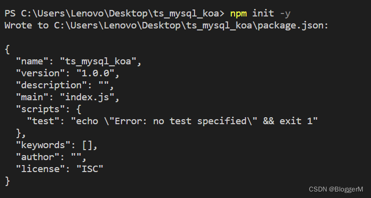
Koa_mySQL_Ts 的整合
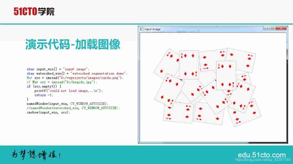
Principle of playing card image segmentation
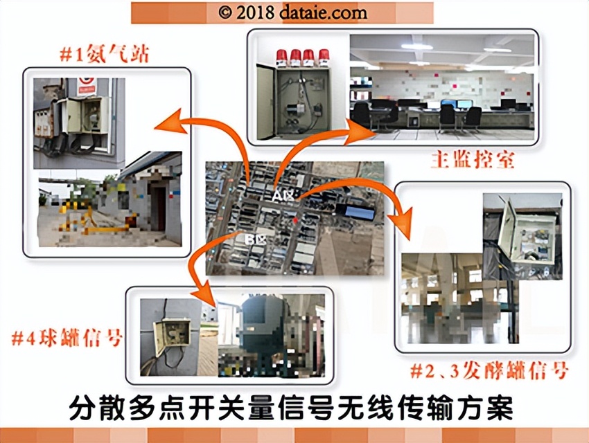
利用无线技术实现分散传感器信号远程集中控制
随机推荐
Opencv learning notes II
opencv学习笔记三
CodeBlocks integrated Objective-C development
leetcode2022年度刷题分类型总结(十二)并查集
golang json unsupported value: NaN 处理
Convex optimization of quadruped
Time functions supported in optee
Discrete device ~ diode triode
GHUnit: Unit Testing Objective-C for the iPhone
批量执行SQL文件
Digital image processing learning (II): Gaussian low pass filter
Method of measuring ripple of switching power supply
Whale conference provides digital upgrade scheme for the event site
Ltp-- extract time, person and place
Diode voltage doubling circuit
Parameter understanding of quad dataloader in yolov5
Learning signal integrity from scratch (SIPI) -- 3 challenges faced by Si and Si based design methods
STM32 project design: temperature, humidity and air quality alarm, sharing source code and PCB
Detailed process of generating URDF file from SW model
Monitor iPad Keyboard Display and hide events