当前位置:网站首页>Kaggle-Titanic
Kaggle-Titanic
2022-07-07 22:17:00 【r1ch4rd】
Recently, I studied kaggle, Did Titanic Project , Use this blog to record
Kaggle-Titanic
kaggle link
Environmental Science :Anaconda,python2.7
github Source link
By looking at the data set , This is a dichotomous problem , So we can use logistic regression model ( The first thought )
Data visualization
First, get the data set, and you need to visually check it to find out the available features .
Feature Engineering ( Very important !!)
1、 Preprocessing
Many data in the data set are incomplete , We need various methods to complete the data set .
① Mode method
Data with few missing items can be filled with modes :
such as Embarked:
#1)Embarked
combined_train_test['Embarked'].fillna(combined_train_test['Embarked'].mode().iloc[0], inplace=True)
② Random forest prediction
Many missing items , But we can use other features to predict the data of this feature as filling :
such as Age:
##6)Age
### Random forest prediction
missing_age_df = pd.DataFrame(combined_train_test[['Age', 'Embarked', 'Sex', 'Title', 'Name_length', 'Fare', 'Fare_bin_id', 'Pclass']])

missing_age_train = missing_age_df[missing_age_df['Age'].notnull()]
missing_age_test = missing_age_df[missing_age_df['Age'].isnull()]
#missing_age_test.info()
from sklearn import ensemble
from sklearn import model_selection
from sklearn.ensemble import GradientBoostingRegressor
from sklearn.ensemble import RandomForestRegressor

def fill_missing_age(missing_age_train, missing_age_test):
    missing_age_X_train = missing_age_train.drop(['Age'], axis=1)
    missing_age_Y_train = missing_age_train['Age']
    missing_age_X_test = missing_age_test.drop(['Age'], axis=1)

    #gbm
    gbm_reg = GradientBoostingRegressor(random_state=42)
    gbm_reg_param_grid = {
   'n_estimators': [2000], 'max_depth': [4], 'learning_rate': [0.01], 'max_features': [3]}
    gbm_reg_grid = model_selection.GridSearchCV(gbm_reg, gbm_reg_param_grid, cv=10, n_jobs=25, verbose=1, scoring='neg_mean_squared_error')
    gbm_reg_grid.fit(missing_age_X_train, missing_age_Y_train)
    print('Age feature Best GB Params:' + str(gbm_reg_grid.best_params_))
    print('Age feature Best GB Score:' + str(gbm_reg_grid.best_score_))
    print('GB Train Error for "Age" Feature Regressor:' + str(
    gbm_reg_grid.score(missing_age_X_train, missing_age_Y_train)))
    missing_age_test.loc[:, 'Age_GB'] = gbm_reg_grid.predict(missing_age_X_test)
    print(missing_age_test['Age_GB'][:4])

    # model 2 rf
    rf_reg = RandomForestRegressor()
    rf_reg_param_grid = {
   'n_estimators': [200], 'max_depth': [5], 'random_state': [0]}
    rf_reg_grid = model_selection.GridSearchCV(rf_reg, rf_reg_param_grid, cv=10, n_jobs=25, verbose=1,
                                               scoring='neg_mean_squared_error')
    rf_reg_grid.fit(missing_age_X_train, missing_age_Y_train)
    print('Age feature Best RF Params:' + str(rf_reg_grid.best_params_))
    print('Age feature Best RF Score:' + str(rf_reg_grid.best_score_))
    print('RF Train Error for "Age" Feature Regressor' + str(
    rf_reg_grid.score(missing_age_X_train, missing_age_Y_train)))
    missing_age_test.loc[:, 'Age_RF'] = rf_reg_grid.predict(missing_age_X_test)
    print(missing_age_test['Age_RF'][:4])

    # two models merge
    print('shape1', missing_age_test['Age'].shape, missing_age_test[['Age_GB', 'Age_RF']].mode(axis=1).shape)
    # missing_age_test['Age'] = missing_age_test[['Age_GB', 'Age_LR']].mode(axis=1)

    missing_age_test.loc[:, 'Age'] = np.mean([missing_age_test['Age_GB'], missing_age_test['Age_RF']])
    print(missing_age_test['Age'][:4])

    missing_age_test.drop(['Age_GB', 'Age_RF'], axis=1, inplace=True)

    return missing_age_test

combined_train_test.loc[(combined_train_test.Age.isnull()), 'Age'] = fill_missing_age(missing_age_train, missing_age_test)
③ The average
For very few missing data with only one or two missing items , Fill in with the average :
combined_train_test['Fare'] = combined_train_test[['Fare']].fillna(combined_train_test.groupby('Pclass').transform(np.mean))2、 Numeric type conversion
because sklearn The requirements in are all digital , Therefore, the non digital type should be transformed :
①dummy
Category variable , such as embarked, Contains only S,C,Q Three variables :
emb_dummies_df = pd.get_dummies(combined_train_test['Embarked'], prefix=combined_train_test[['Embarked']].columns[0])②factorize
dummy Can't handle it very well Cabin In this way, there are many attributes with variables ,factorize() You can create some numbers , To represent a variable , Map one for each category ID, This mapping finally produces only one feature , Don't like dummy Generate multiple features : To be improved
③scaling
It's a mapping , Map larger values to smaller ranges , such as (-1,1).
Age The scope of is much larger than that of other attributes , This makes Age There will be greater weight , We need to scaling( Feature scaling )
from sklearn import preprocessing
assert np.size(df['Age']) == 891
scaler = preprocessing.StandardScaler()
df['Age_scaled'] = scaler.fit_transform(df['Age'].values.reshape(-1, 1))
④Binning
Fare Attribute processing can also use the above method scaling, It can also be used. binning. This is a method of discretizing continuous data , Divide the value into the set range ( bucket ) in .
combined_train_test['Fare_bin'] = pd.qcut(combined_train_test['Fare'], 5)Of course, data bin After melting , must factorize perhaps dummy.
combined_train_test['Fare_bin_id'] = pd.factorize(combined_train_test['Fare_bin'])[0]

fare_bin_dummies_df = pd.get_dummies(combined_train_test['Fare_bin_id']).rename(columns = lambda x: 'Fare_' + str(x))
combined_train_test = pd.concat([combined_train_test,fare_bin_dummies_df], axis=1)
combined_train_test.drop(['Fare_bin'], axis=1, inplace=True)
3、 Discard useless features
Throw in some of the previously processed tag attributes , Or labels produced halfway , And useless labels for models .
After correlation analysis and cross validation , Add useful tags .
# Discard useless features
combined_data_backup = combined_train_test
combined_train_test.drop(['PassengerId', 'Embarked', 'Sex', 'Name', 'Title', 'Fare_bin_id', 'Pclass_Fare_Category',
                       'Parch', 'SibSp', 'Ticket', 'Family_Size_Category'],axis=1,inplace=True)
Build a model
Establish a simple logistic regression model :
from sklearn import linear_model

clf = linear_model.LogisticRegression(C=1.0, penalty='l1', tol=1e-6)
clf.fit(titanic_train_data_X.values, titanic_train_data_Y.values)

#print clf

predictions = clf.predict(titanic_test_data_X)
result = pd.DataFrame({
   'PassengerId':test_df_org['PassengerId'].values, 'Survived':predictions.astype(np.int32)})
result.to_csv("~/Documents/data/base_line_predictions.csv", index=False)
Cross validation
Use the original data set for cross validation ( To be improved )
correlation analysis
Pit to be filled
Model fusion
bagging Methods model fusion :
from sklearn.ensemble import BaggingRegressor

# fit To BaggingRegressor In
clf = linear_model.LogisticRegression(C=1.0, penalty='l1', tol=1e-6)
bagging_clf = BaggingRegressor(clf, n_estimators=20, max_samples=0.8, max_features=1.0, bootstrap=True,
                               bootstrap_features=False, n_jobs=-1)
bagging_clf.fit(titanic_train_data_X.values, titanic_train_data_Y.values)

predictions = bagging_clf.predict(titanic_test_data_X)
result = pd.DataFrame({
   'PassengerId': test_df_org['PassengerId'].values, 'Survived': predictions.astype(np.int32)})
result.to_csv("~/Documents/data/base_bagging_predictions.csv", index=False)
Catalog
边栏推荐
- Use br to recover backup data on azure blob storage
- Automatic classification of defective photovoltaic module cells in electronic images
- The whole network "chases" Zhong Xuegao
- Paint basic graphics with custompaint
- [colmap] sparse reconstruction is converted to mvsnet format input
- Prometheus remote_ write InfluxDB,unable to parse authentication credentials,authorization failed
- OpenGL configuration vs2019
- OpenGL jobs - shaders
- Solve the problem of uni in uni app Request sent a post request without response.
- South China x99 platform chicken blood tutorial
猜你喜欢
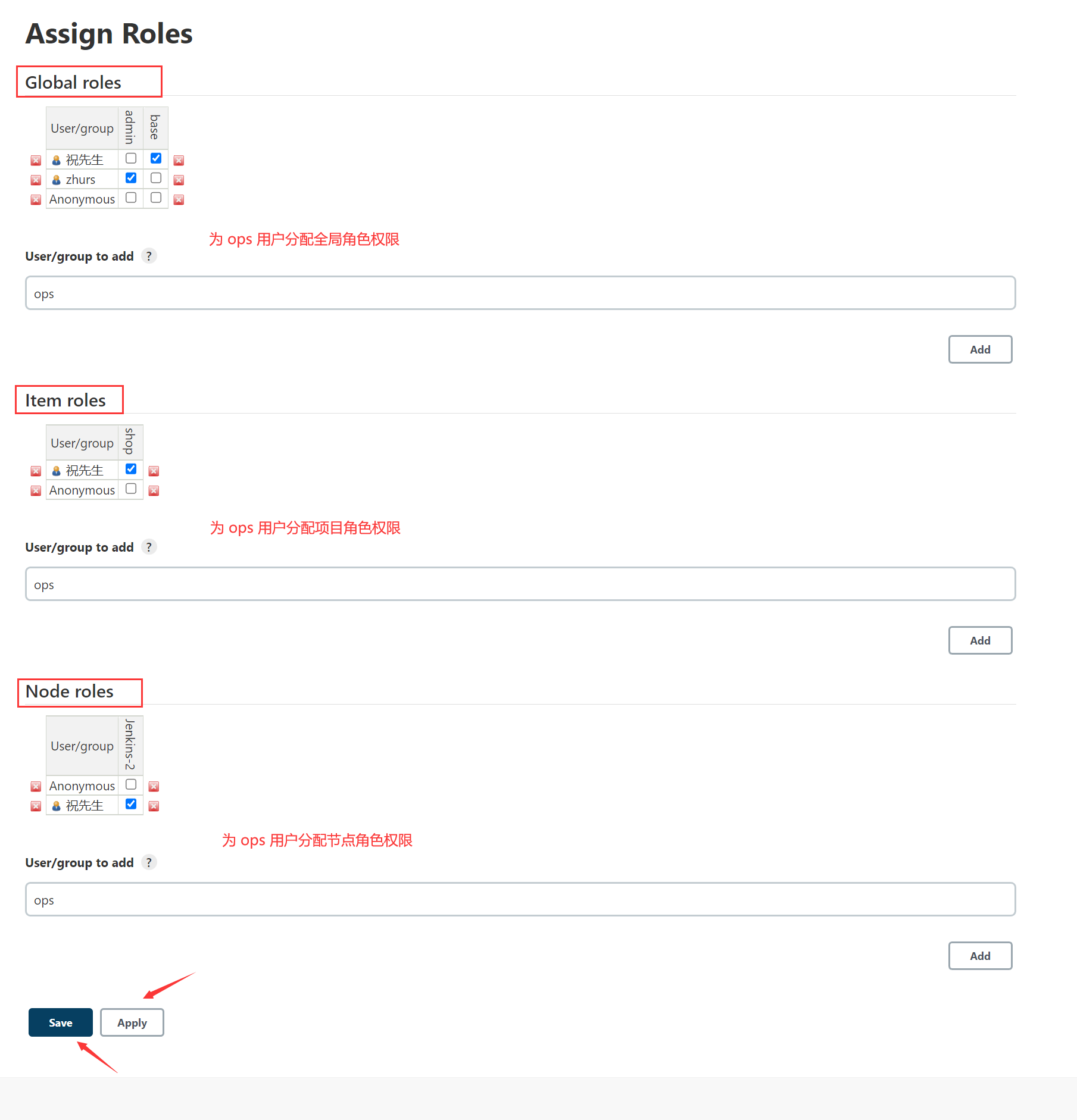
Jenkins user rights management
![Jerry's about TWS channel configuration [chapter]](/img/94/fde5054fc412b786cd9864215e912c.png)
Jerry's about TWS channel configuration [chapter]

使用 BlocConsumer 同时构建响应式组件和监听状态

An overview of the latest research progress of "efficient deep segmentation of labels" at Shanghai Jiaotong University, which comprehensively expounds the deep segmentation methods of unsupervised, ro
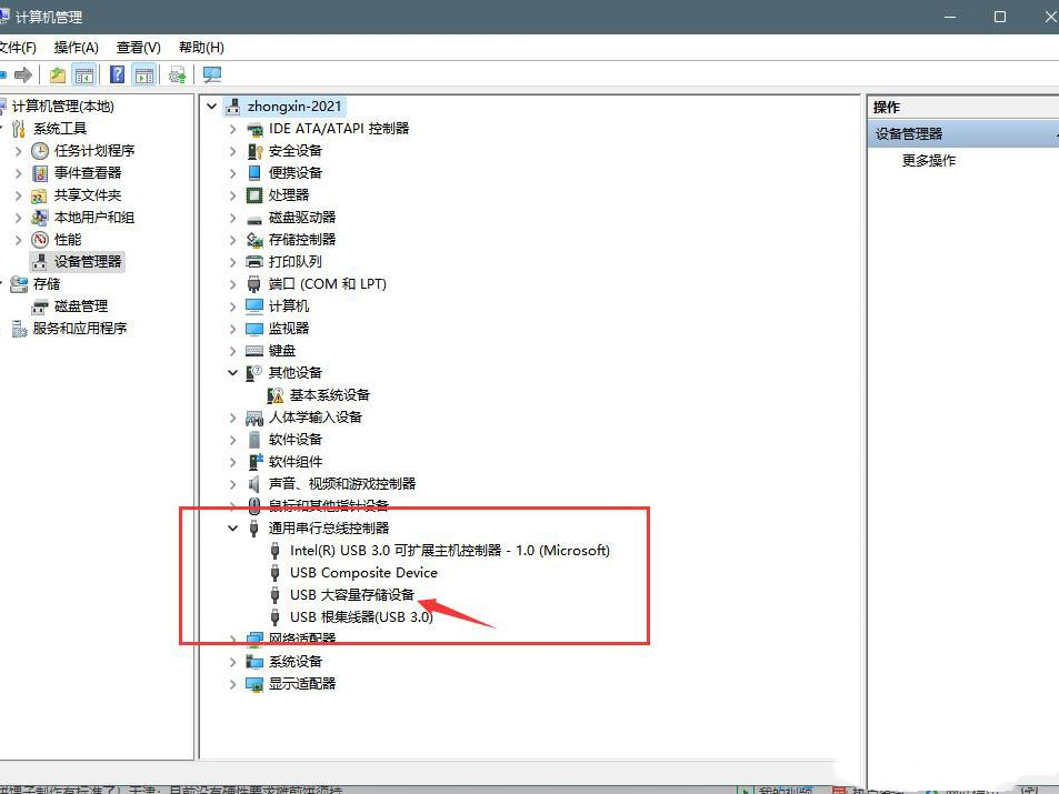
What if the win11u disk does not display? Solution to failure of win11 plug-in USB flash disk
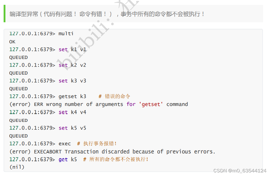
Redis - basic use (key, string, list, set, Zset, hash, geo, bitmap, hyperloglog, transaction)

【Azure微服务 Service Fabric 】因证书过期导致Service Fabric集群挂掉(升级无法完成,节点不可用)

Index summary (assault version)
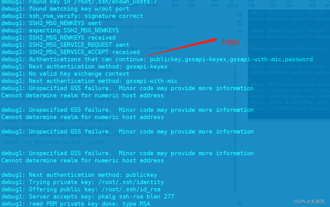
Debugging and handling the problem of jamming for about 30s during SSH login

Google SEO external chain backlinks research tool recommendation
随机推荐
Pre sale 179000, hengchi 5 can fire? Product power online depends on how it is sold
PKPM 2020 software installation package download and installation tutorial
2022 how to evaluate and select low code development platforms?
Win11U盘不显示怎么办?Win11插U盘没反应的解决方法
ByteDance Android interview, summary of knowledge points + analysis of interview questions
TCP/IP 协议栈
How does win11 unblock the keyboard? Method of unlocking keyboard in win11
How to integrate Google APIs with Google's application system (1) -introduction to Google APIs
null == undefined
Jerry's manual matching method [chapter]
23. Merge K ascending linked lists -c language
How to make agile digital transformation strategy for manufacturing enterprises
South China x99 platform chicken blood tutorial
The function is really powerful!
NVR hard disk video recorder is connected to easycvr through the national standard gb28181 protocol. What is the reason why the device channel information is not displayed?
The cyberspace office announced the measures for data exit security assessment, which will come into force on September 1
如何实现横版游戏中角色的移动控制
SAR影像质量评估
Application practice | the efficiency of the data warehouse system has been comprehensively improved! Data warehouse construction based on Apache Doris in Tongcheng digital Department
嵌入式开发:如何为项目选择合适的RTOS?