当前位置:网站首页>Fundamentals of deep learning convolutional neural network (CNN)
Fundamentals of deep learning convolutional neural network (CNN)
2022-07-05 19:43:00 【Falling flowers and rain】
List of articles
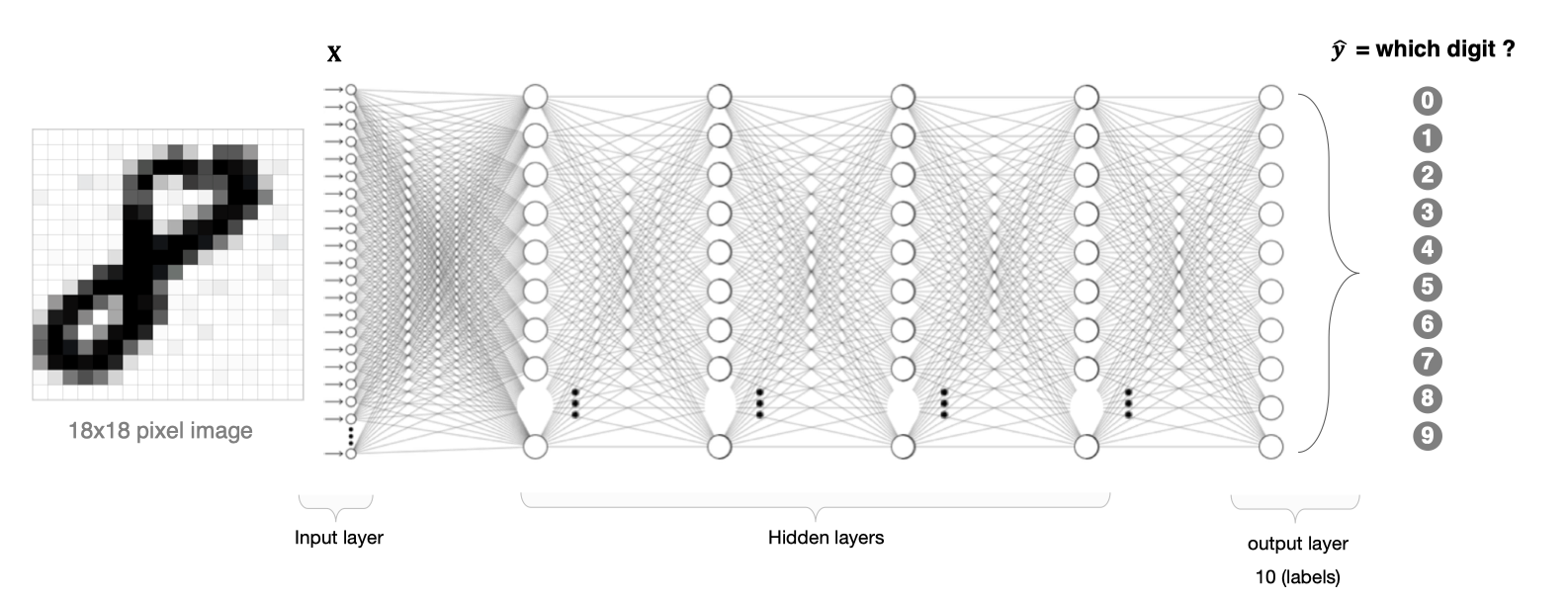
There are two problems in image processing using fully connected neural network :
- A large amount of data needs to be processed , Low efficiency
If we deal with one 1000×1000 Pixel image , The parameters are as follows :
1000×1000×3=3,000,000
Such a large amount of data processing is very resource consuming
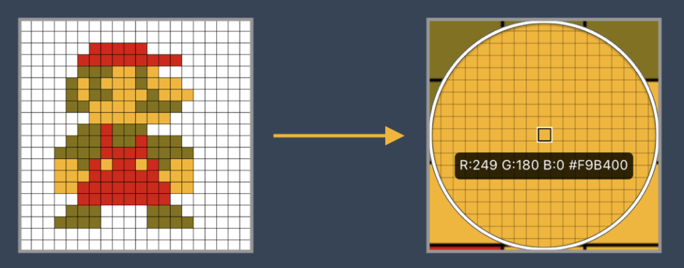
- It is difficult to retain the original features in the process of image dimension adjustment , The accuracy of image processing is not high
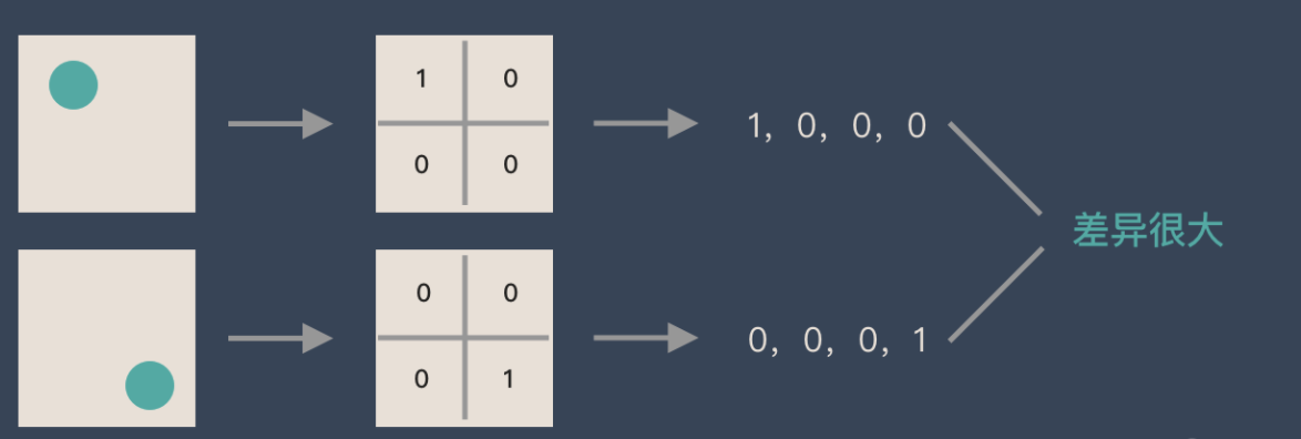
If there is a circle, it is 1, No circle is 0, Then different positions of the circle will produce completely different data expressions . But from an image point of view , The content of the image ( The essence ) Nothing has changed , It's just that the position has changed . So when we move the object in the image , The results obtained with full connection lifting will be very different , This is not in line with the requirements of image processing .
1. CNN The composition of the network
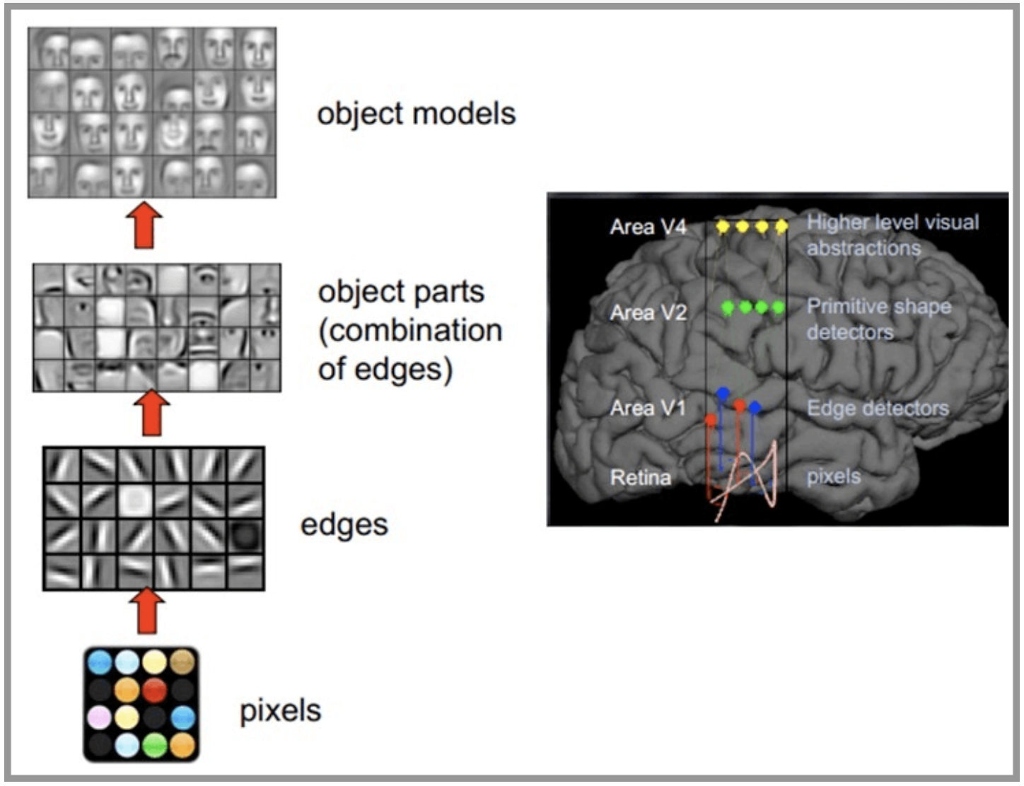
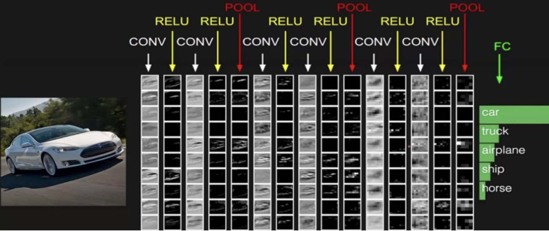
CNN The network is inspired by the human visual nervous system , The principle of human vision : Start with the raw signal intake ( Pupil intake pixels Pixels), Then do the preliminary treatment ( Some cells in the cortex find the edge and direction ), Then abstract ( The brain decides , The shape of the object in front of us , It's round ), And then further abstract ( The brain further determines that the object is a face ). Here is an example of human face recognition :
CNN The network is mainly composed of three parts : Convolution layer 、 Pool layer and full connection layer , The convolution layer is responsible for extracting local features in the image ; The pool layer is used to greatly reduce the parameter magnitude ( Dimension reduction ); The whole connection layer is similar to the part of artificial neural network , Used to output the desired result .

Whole CNN The network structure is shown in the figure below :
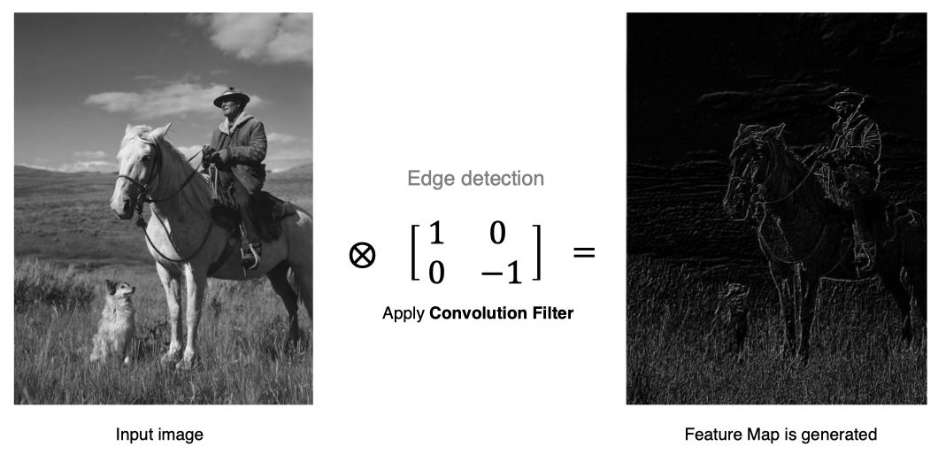
2. Convolution layer
Convolution layer is the core module of convolution neural network , The purpose of convolution layer is to extract the features of input feature map , As shown in the figure below , Convolution kernel can extract the edge information in the image .
2.1 Calculation method of convolution
How is convolution calculated ?
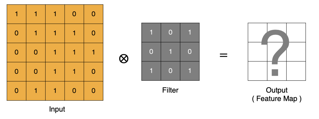
Convolution is essentially a dot product between the filter and the local area of the input data .
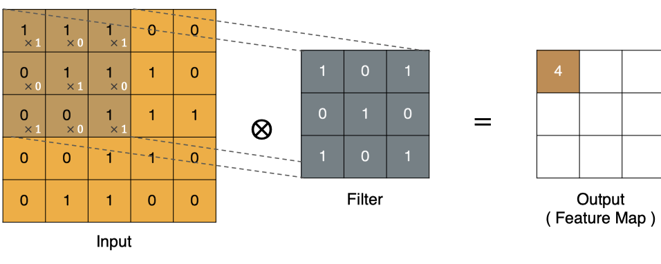
The calculation method of the point in the upper left corner :

Similarly, other points can be calculated , Get the final convolution result ,
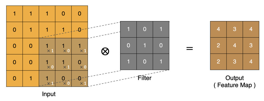
The last point is calculated by :

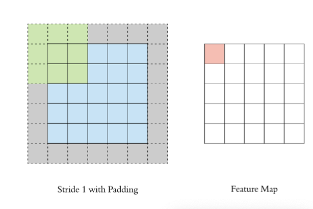
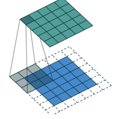
2.2 padding
In the above convolution process , The feature graph is much smaller than the original graph , We can do it around the original image padding, To ensure that the size of the characteristic image remains unchanged in the convolution process .
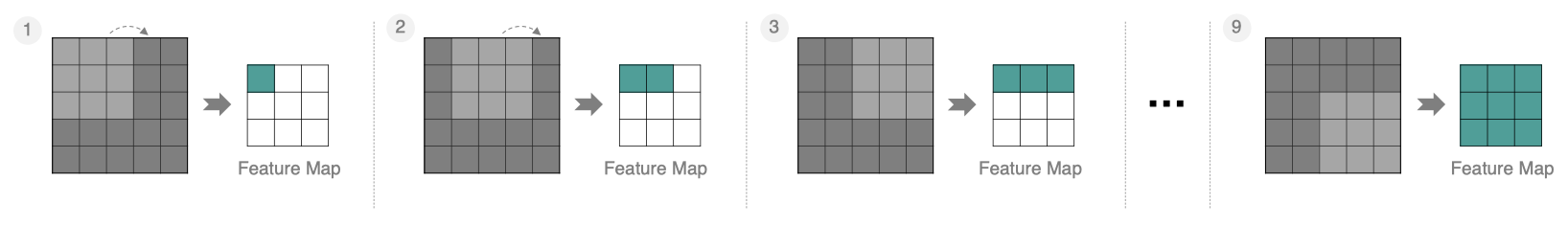
2.3 stride
In steps of 1 To move the convolution kernel , The calculated characteristic diagram is as follows :
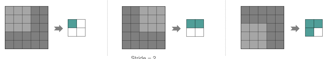
If we put stride increase , Let's set it to 2, It can also extract feature map , As shown in the figure below :
2.4 Multichannel convolution
In practice, images are composed of multiple channels , How do we compute convolution ?
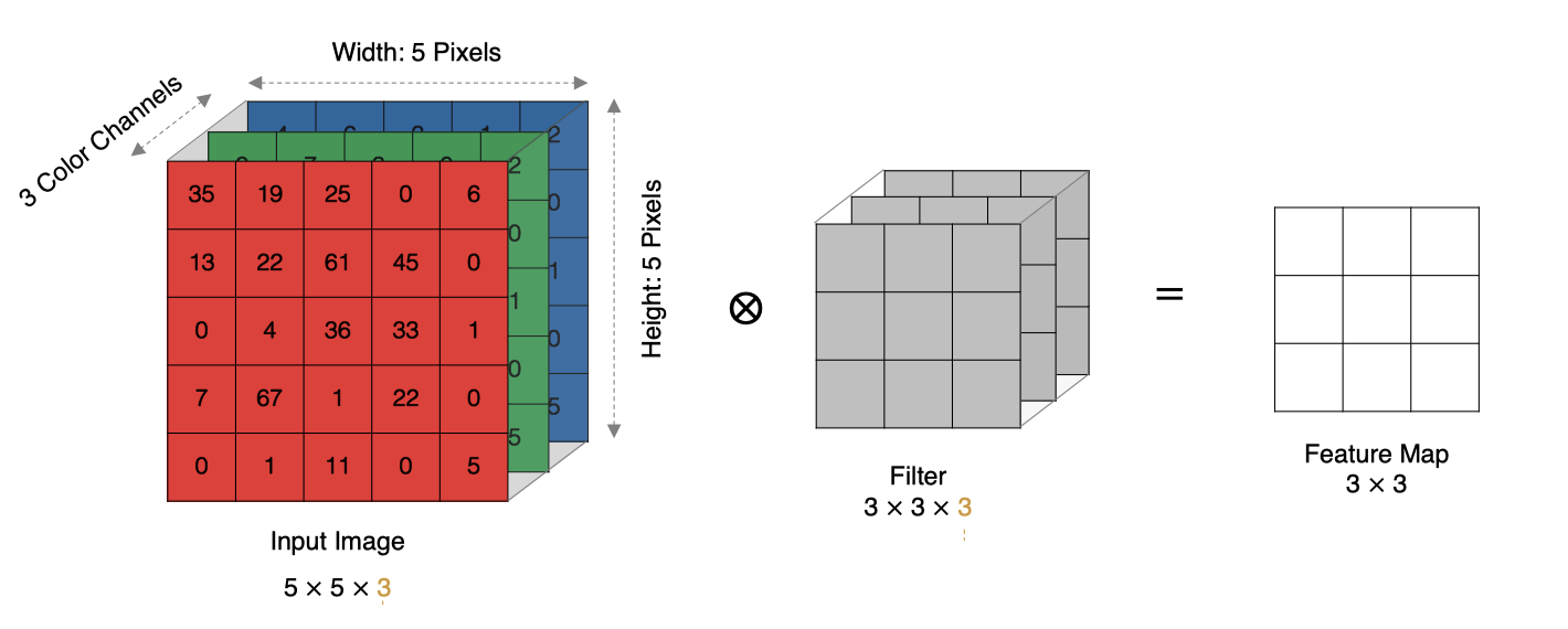
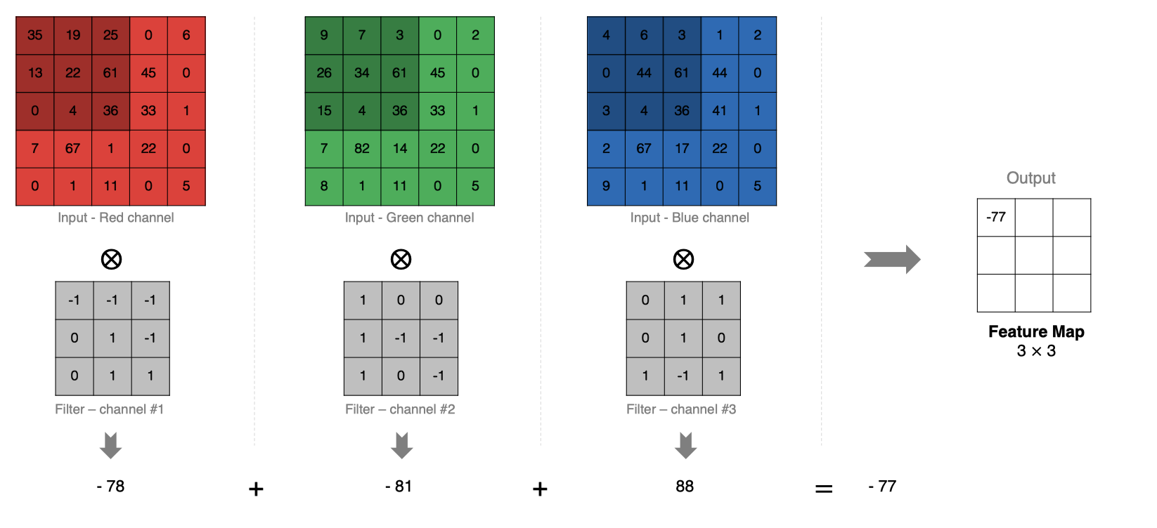
The calculation method is as follows : When the input has multiple channels (channel) when ( For example, pictures can have RGB Three channels ), Convolution kernels need to have the same channel Count , Every convolution kernel channel Corresponding to the input layer channel Convolution , Each one channel The convolution results are added bit by bit to obtain the final Feature Map
2.5 Multi convolution kernel convolution
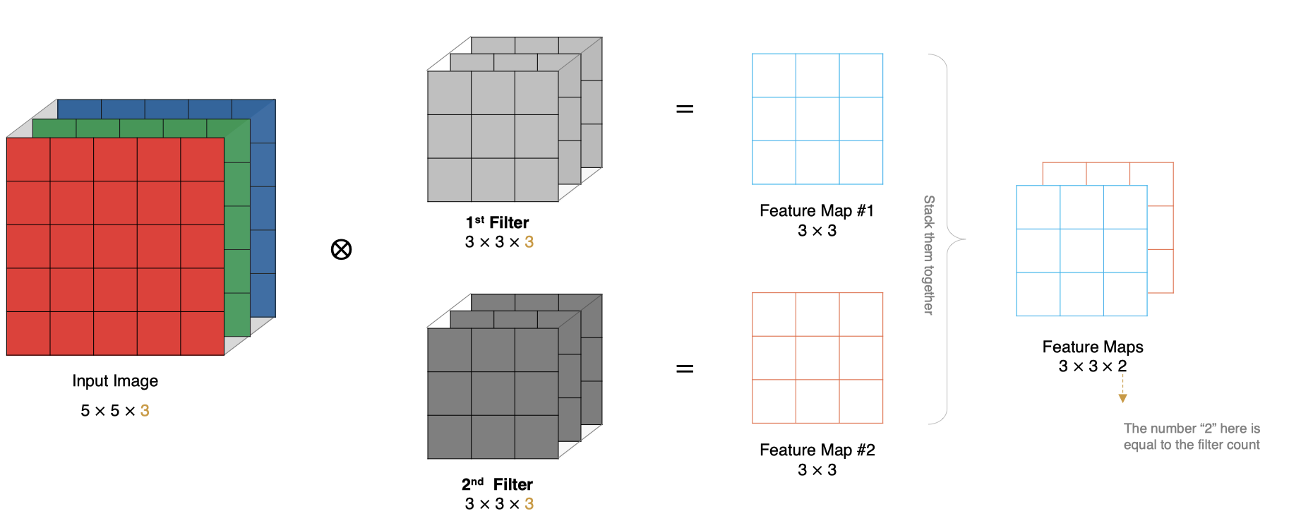
How to calculate if there are multiple convolution kernels ? When there are multiple convolution kernels , Each convolution kernel learns different features , The corresponding generation contains multiple channel Of Feature Map, For example, the following figure has two filter, therefore output There are two channel.
2.6 Feature map size
The size of the output feature map is closely related to the following parameters : * size: Convolution kernel / Filter size , It is usually odd , Such as the 1 * 1, 3 * 3, 5 * 5 * padding: The way of zero filling * stride: step
The calculation method is shown in the figure below :
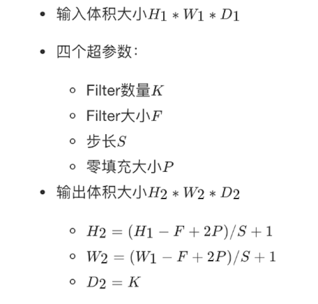
The input characteristic graph is 5x5, Convolution kernels for 3x3, Plus padding by 1, Then its output size is :
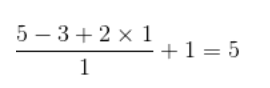
As shown in the figure below :
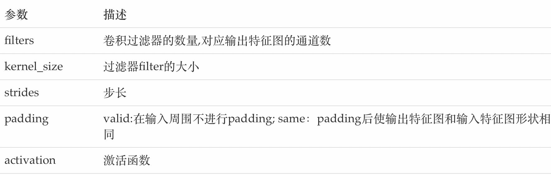
stay tf.keras The implementation of convolution kernel in
tf.keras.layers.Conv2D(
    filters, kernel_size, strides=(1, 1), padding='valid',
     activation=None
)
The main parameters are as follows :
3. Pooling layer (Pooling)
The pooling layer reduces the input dimension of subsequent network layers , Reduce the size of the model , Speed up the calculation , And improved. Feature Map The robustness of , Prevent over fitting ,
It mainly down samples the feature map learned by the convolution layer (subsampling) Handle , It mainly consists of two
3.1 Maximum pooling
Max Pooling, Take the maximum value in the window as the output , This method is widely used .

stay tf.keras The method implemented in is :
tf.keras.layers.MaxPool2D(
    pool_size=(2, 2), strides=None, padding='valid'
)
Parameters :
pool_size:  The size of the pooled window

strides:  Step size of window movement , The default is 1

padding:  Whether to fill , The default is no filling
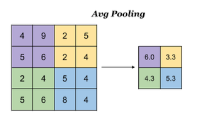
3.2 The average pooling
Avg Pooling, Take the average value of all values in the window as the output
stay tf.keras The way to implement pooling in is :
tf.keras.layers.AveragePooling2D(
    pool_size=(2, 2), strides=None, padding='valid'
)
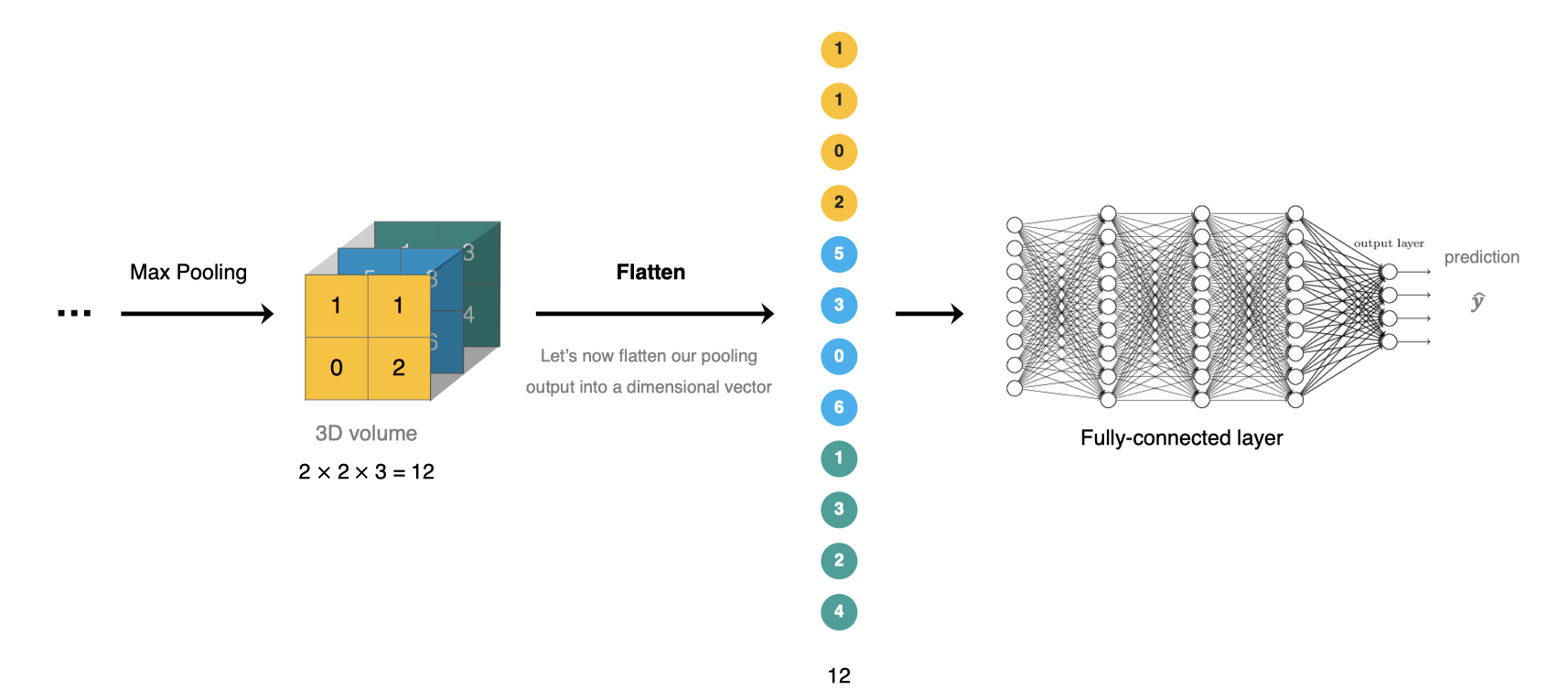
4. Fully connected layer
The full connection layer is located at CNN The end of the network , After feature extraction of convolution layer and dimension reduction of pool layer , The operation of transforming the feature map into a one-dimensional vector and sending it to the full connection layer for classification or regression .
stay tf.keras In the whole connection layer tf.keras.dense Realization .
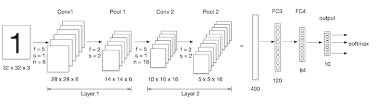
5. Construction of convolutional neural network
We construct convolutional neural networks in mnist Processing on data sets , As shown in the figure below :LeNet-5 It's a simple convolutional neural network , Input 2D image , First pass through two convolutions , Pooling layer , And then through the full connection layer , Finally using softmax Classification as the output layer .
Import toolkit :
import tensorflow as tf
#  Data sets
from tensorflow.keras.datasets import mnist
5.1 Data loading
Consistent with the case of neural network , First load the dataset :
(train_images, train_labels), (test_images, test_labels) = mnist.load_data()
5.2 Data processing
The input requirements of convolutional neural network are :NHWC , They are the number of pictures , Picture height , Picture width and picture channel , Because it's grayscale , Passageway is 1.
#  Data processing :num,h,w,c
#  Training set data
train_images = tf.reshape(train_images, (train_images.shape[0],train_images.shape[1],train_images.shape[2], 1))
print(train_images.shape)
#  Test set data
test_images = tf.reshape(test_images, (test_images.shape[0],test_images.shape[1],test_images.shape[2], 1))
The result is :
(60000, 28, 28, 1)
5.3 Model structures,
Lenet-5 Two dimensional image of model input , First pass through two convolutions , Pooling layer , And then through the full connection layer , Finally using softmax Classification as the output layer , The model is constructed as follows :
#  model building
net = tf.keras.models.Sequential([
    #  Convolution layer :6 individual 5*5 Convolution kernel , Activation is sigmoid
      tf.keras.layers.Conv2D(filters=6,kernel_size=5,activation='sigmoid',input_shape=  (28,28,1)),
    #  Maximum pooling
    tf.keras.layers.MaxPool2D(pool_size=2, strides=2),
    #  Convolution layer :16 individual 5*5 Convolution kernel , Activation is sigmoid
    tf.keras.layers.Conv2D(filters=16,kernel_size=5,activation='sigmoid'),
    #  Maximum pooling
    tf.keras.layers.MaxPool2D(pool_size=2, strides=2),
    #  Dimension adjusted to 1 D data
    tf.keras.layers.Flatten(),
    #  Full convolution , Activate sigmoid
    tf.keras.layers.Dense(120,activation='sigmoid'),
    #  Full convolution , Activate sigmoid
    tf.keras.layers.Dense(84,activation='sigmoid'),
    #  Full convolution , Activate softmax
    tf.keras.layers.Dense(10,activation='softmax')

])
We go through net.summary() Look at the network structure :
Model: "sequential_11"
_________________________________________________________________
Layer (type)                 Output Shape              Param #
=================================================================
conv2d_4 (Conv2D)            (None, 24, 24, 6)         156
_________________________________________________________________
max_pooling2d_4 (MaxPooling2 (None, 12, 12, 6)         0
_________________________________________________________________
conv2d_5 (Conv2D)            (None, 8, 8, 16)          2416
_________________________________________________________________
max_pooling2d_5 (MaxPooling2 (None, 4, 4, 16)          0
_________________________________________________________________
flatten_2 (Flatten)          (None, 256)               0
_________________________________________________________________
dense_25 (Dense)             (None, 120)               30840
_________________________________________________________________
dense_26 (Dense)             (None, 84)                10164

dense_27 (Dense)             (None, 10)                850
=================================================================
Total params: 44,426
Trainable params: 44,426
Non-trainable params: 0
______________________________________________________________
The size of the handwritten digital input image is 28x28x1, Here's the picture , Let's look at the parameters of the lower convolution :
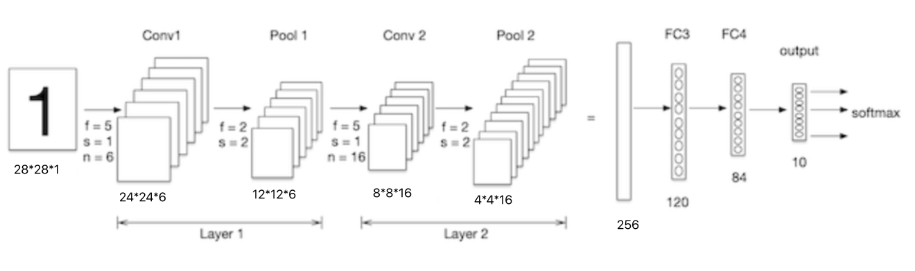
conv1 The convolution kernel in is 5x5x1, The number of convolution kernels is 6, Each convolution kernel has one bias, So the parameter quantity is :5x5x1x6+6=156.
conv2 The convolution kernel in is 5x5x6, The number of convolution kernels is 16, Each convolution kernel has one bias, So the parameter quantity is :5x5x6x16+16 = 2416.
5.4 Model compilation
Set optimizer and loss function :
#  Optimizer
optimizer = tf.keras.optimizers.SGD(learning_rate=0.9)
#  Model compilation : Loss function , Optimizer and evaluation index
net.compile(optimizer=optimizer,
              loss='sparse_categorical_crossentropy',
              metrics=['accuracy'])
5.5 model training
model training :
#  model training
net.fit(train_images, train_labels, epochs=5, validation_split=0.1)
The training process :
Epoch 1/5
1688/1688 [==============================] - 10s 6ms/step - loss: 0.8255 - accuracy: 0.6990 - val_loss: 0.1458 - val_accuracy: 0.9543
Epoch 2/5
1688/1688 [==============================] - 10s 6ms/step - loss: 0.1268 - accuracy: 0.9606 - val_loss: 0.0878 - val_accuracy: 0.9717
Epoch 3/5
1688/1688 [==============================] - 10s 6ms/step - loss: 0.1054 - accuracy: 0.9664 - val_loss: 0.1025 - val_accuracy: 0.9688
Epoch 4/5
1688/1688 [==============================] - 11s 6ms/step - loss: 0.0810 - accuracy: 0.9742 - val_loss: 0.0656 - val_accuracy: 0.9807
Epoch 5/5
1688/1688 [==============================] - 11s 6ms/step - loss: 0.0732 - accuracy: 0.9765 - val_loss: 0.0702 - val_accuracy: 0.9807
5.6 Model to evaluate
#  Model to evaluate
score = net.evaluate(test_images, test_labels, verbose=1)
print('Test accuracy:', score[1])
Output is :
313/313 [==============================] - 1s 2ms/step - loss: 0.0689 - accuracy: 0.9780
Test accuracy:  0.9779999852180481
Compared with using a fully connected network , Accuracy has improved a lot .
边栏推荐
- UWB超宽带定位技术,实时厘米级高精度定位应用,超宽带传输技术
- third-party dynamic library (libcudnn.so) that Paddle depends on is not configured correctl
- JMeter 常用的几种断言方法,你会了吗?
- What is the function of okcc call center
- Is it safe for Guohai Securities to open an account online?
- MMO項目學習一:預熱
- Relationship between floating elements and parent and brother boxes
- 面试官:Redis中集合数据类型的内部实现方式是什么?
- 完爆面试官,一线互联网企业高级Android工程师面试题大全
- How about testing outsourcing companies?
猜你喜欢
webuploader文件上传 拖拽上传 进度监听 类型控制 上传结果监听控件
Postman核心功能解析-参数化和测试报告
![[OBS] qstring's UTF-8 Chinese conversion to blog printing UTF-8 char*](/img/cc/172684664a9115943d45b0646ef110.png)
[OBS] qstring's UTF-8 Chinese conversion to blog printing UTF-8 char*

UWB超宽带定位技术,实时厘米级高精度定位应用,超宽带传输技术
Django使用mysqlclient服务连接并写入数据库的操作过程
JAD installation, configuration and integration idea
40000 word Wenshuo operator new & operator delete
Summer Challenge database Xueba notes, quick review of exams / interviews~
Apprentissage du projet MMO I: préchauffage
Redis cluster simulated message queue
随机推荐
Fuzor 2020軟件安裝包下載及安裝教程
全网最全的低代码/无代码平台盘点:简道云、伙伴云、明道云、轻流、速融云、集简云、Treelab、钉钉·宜搭、腾讯云·微搭、智能云·爱速搭、百数云
Django使用mysqlclient服务连接并写入数据库的操作过程
No matter how busy you are, you can't forget safety
四万字长文说operator new & operator delete
太牛了,看这篇足矣了
MMO项目学习一:预热
手机开户选择哪家券商公司比较好哪家平台更安全
不愧是大佬,字节大牛耗时八个月又一力作
如何安全快速地从 Centos迁移到openEuler
城链科技数字化创新战略峰会圆满召开
【C语言】字符串函数及模拟实现strlen&&strcpy&&strcat&&strcmp
【obs】libobs-winrt :CreateDispatcherQueueController
大厂面试必备技能,2022Android不死我不倒
[Collection - industry solutions] how to build a high-performance data acceleration and data editing platform
Worthy of being a boss, byte Daniel spent eight months on another masterpiece
【硬核干货】数据分析哪家强?选Pandas还是选SQL
How MySQL queries and modifies JSON data
Reinforcement learning - learning notes 4 | actor critical
C#应用程序界面开发基础——窗体控制(5)——分组类控件