当前位置:网站首页>1.20 study univariate linear regression
1.20 study univariate linear regression
2022-06-26 08:47:00 【Thick Cub with thorns】
1.20 study
List of articles
One 、 introduction (Introduction)
List of articles
1.1 welcome
But in fact, I only know the algorithm 、 Math doesn't solve the practical problems you care about . therefore , We will spend a lot of time doing exercises , So you can implement each of these algorithms yourself , So as to understand the internal mechanism .
that , Why is machine learning so popular ? as a result of , Machine learning is not just used in the field of artificial intelligence .
Finally, learning algorithms are used to understand human learning and understand the brain .
In the next video , We will begin to give a more formal definition , What is machine learning . Then we will start to learn the main problems and algorithms of machine learning. You will know some main machine learning terms , And start to understand different algorithms , Which algorithm is more appropriate .
1.2 What is machine learning ?
The first definition of machine learning comes from Arthur Samuel. He defined machine learning as , In the case of specific programming , Areas that give computer learning ability .Samuel The definition of can be traced back to 50 years , He wrote a chess program . The magic of this program is , The programmer himself is not a chess player . But because he's too good , So through programming , Let the chess program play tens of thousands of chess with itself . By observing which layout ( Chessboard position ) It will win , Which layout will lose , in the course of time , This chess program understands what a good layout is , What is a bad layout . And then it's crazy , After learning the program , The level of playing chess exceeds Samuel. This is definitely a remarkable achievement .
Another more recent definition , from Tom Mitchell Put forward , From Carnegie Mellon University ,Tom The definition of machine learning is , A good learning problem is defined as follows , He said ,== A program is thought to be able to learn from experience E Middle school learning , Solve the task T, Performance metrics reached P, If and only if , Experience gained E after , after P judge , The program is processing T Improved performance when .== I think experience E It is the experience and task of tens of thousands of self-practice procedures T Is playing chess . Performance metrics P Well , It's when it plays against some new opponents , Probability of winning the game .
In this lesson , I want to teach you about different types of learning algorithms . There are several different types of learning algorithms . The two main types are called supervised learning and unsupervised learning . In the next few videos , I will give the definitions of these terms . Here are two simple sentences , The idea of supervised learning means , We will teach computers how to complete tasks , And in unsupervised learning , We intend to let it learn by itself . If you are still confused about these two terms , Please don't worry , In the next two videos , I will introduce these two learning algorithms in detail .
This is machine learning , These are the topics I want to teach . In the next video , I will define what supervised learning is , What is unsupervised learning . Besides , Explore when to use both .
1.3 Supervised learning
Reference video : 1 - 3 - Supervised Learning (12 min).mkv
In this video , I want to define what is probably the most common machine learning problem : That is supervised learning . I will formally define supervised learning later .
Let's use an example to introduce what is supervised learning. The formal definition is introduced later . If you want to predict house prices .
A while ago , A student collected data on house prices from a research institute in Portland, Oregon . You draw these data , It looks like this : The horizontal axis represents the area of the house , The unit is square feet , The vertical axis represents house prices , The unit is thousands of dollars . Based on this set of data , If you have a friend , He has a set of 750 Square foot house , Now he wants to sell his house , He wants to know how much the house can sell .
So about this question , How will machine learning algorithms help you ?
[ Failed to transfer the external chain picture , The origin station may have anti-theft chain mechanism , It is suggested to save the pictures and upload them directly (img-ihdVcnyl-1642651282898)(…/images/2d99281dfc992452c9d32e022ce71161.png)]
We apply learning algorithms , You can draw a straight line in this set of data , Or to put it another way , Fit a straight line , From this line, we can infer , The house may sell $$150,000 , When however this No yes only One Of count Law . can can also Yes more good Of , Than Such as I People No use straight Line quasi close this some Count According to the , use Two Time Fang cheng Go to quasi close can can effect fruit Meeting more good . root According to the Two Time Fang cheng Of song Line , I People can With from this individual spot PUSH measuring Out , this set room Son can sell Pick up near , Of course, this is not the only algorithm . Maybe there's something better , For example, we don't use straight lines to fit these data , It may be better to use quadratic equation to fit . According to the curve of quadratic equation , We can deduce from this point , The house can sell close to , When however this No yes only One Of count Law . can can also Yes more good Of , Than Such as I People No use straight Line quasi close this some Count According to the , use Two Time Fang cheng Go to quasi close can can effect fruit Meeting more good . root According to the Two Time Fang cheng Of song Line , I People can With from this individual spot PUSH measuring Out , this set room Son can sell Pick up near $200,000$. Later we will discuss how to choose a learning algorithm , How to decide whether to use a straight line or a quadratic equation to fit . One of the two options can make your friend's house sell more reasonably . These are good examples of learning algorithms . The above is an example of supervised learning .
It can be seen that , Supervised learning means that we give the learning algorithm a data set . By this data set “ right key ” form . In the case of house prices , We gave a series of house data , We give the correct price for each sample in a given dataset , That's how much they actually sell, and then using learning algorithms , Work out more correct answers . For example, the price of your friend's new house . In terms of terms , It's called The return question . We Try to guess the result of a continuous value , The price of the house .
Generally, the price of a house will be recorded in cents , So house prices are actually a series of discrete values , But we usually regard house prices as real numbers , As a scalar , So we think of it as a continuous number .
The word return means , We are trying to infer this series of continuous value attributes .
Let me give another example of supervised learning . I have studied this before with some friends . Suppose you want to guess whether breast cancer is benign or not by looking at medical records. , If someone detects a breast tumor , Malignant tumors are harmful and dangerous , Benign tumors are less harmful , So people obviously care about this problem .
[ Failed to transfer the external chain picture , The origin station may have anti-theft chain mechanism , It is suggested to save the pictures and upload them directly (img-kuh1bFyd-1642651282901)(…/images/4f80108ebbb6707d39b7a6da4d2a7a4e.png)]
Let's look at a set of data : This dataset , The horizontal axis shows the size of the tumor , On the longitudinal axis , I marked 1 and 0 Indicates whether it is a malignant tumor or not . The tumors we've seen before , If it is malignant, it is recorded as 1, Not malignant , Or benign as 0.
I have a 5 Benign tumor samples , stay 1 The location of this is 5 A malignant tumor sample . Now we have a friend who unfortunately has a breast tumor . Suppose her tumor is about this big , So the problem with machine learning is , Can you estimate the probability that the tumor is malignant or benign . In terms of terms , This is a question of classification .
Classification refers to , We're trying to figure out the discrete output :0 or 1 Benign or malignant , In fact, in the problem of classification , The output may have more than two values . For example, there may be three types of breast cancer , So you want to predict discrete output 0、1、2、3.0 Represents good ,1 It means the first one 1 Breast cancer ,2 It means the first one 2 Carcinoid ,3 It means the first one 3 class , But this is also a classification problem .
Because these discrete outputs correspond to benign signals respectively , Type I, type II or type III cancer , In the classification problem, we can draw these data points in another way .
Now I use different symbols to represent these data . Since we regard the size of the tumor as a feature to distinguish malignant from benign , Then I can draw like this , I use different symbols to represent benign and malignant tumors . Or negative samples and positive samples. Now we don't draw all of them X, Benign tumors are replaced with O Express , Malignant continue to use X Express . To predict whether the tumor is malignant or not .
In some other machine learning problems , More than one feature may be encountered . for instance , We don't just know the size of the tumor , Also know the age of the corresponding patient . In other machine learning problems , We usually have more characteristics , When my friend studied this problem , These features are usually used , Such as mass density , Consistency of tumor cell size and shape, etc , There are other features . This is one of the most interesting learning algorithms we are about to learn .
That algorithm can not only handle 2 Kind of 3 To plant or 5 Species characteristics , Even an infinite number of features can be processed .
[ Failed to transfer the external chain picture , The origin station may have anti-theft chain mechanism , It is suggested to save the pictures and upload them directly (img-qZ3s2c2f-1642651282902)(…/images/c34fa10153f223aa955d6717663a9f91.png)]
Above picture , I listed a total of 5 Different characteristics , Two on the axis and one on the right 3 Kind of , But in some learning problems , You wish you didn't just 3 To plant or 5 Species characteristics . contrary , You want to use an infinite variety of features , So that your algorithm can take advantage of a large number of features , Or clues to speculate . How do you deal with infinite features , Even how to store these features is problematic , Your computer certainly doesn't have enough memory .== We'll talk about an algorithm later , It's called support vector machine , There is a clever mathematical skill , It allows the computer to process an infinite number of features .== Imagine , I didn't write down these two and the three features on the right , But in an infinitely long list , Keep writing, keep writing , Write down an infinite number of features , in fact , We can use algorithms to deal with them .
Now let's review , In this lesson, we introduced supervised learning . The basic idea is this ,== Each sample in our dataset has a corresponding “ right key ”. And then make predictions based on these samples ,== As in the case of houses and tumors . We also introduce the regression problem , That is, a continuous output is derived by returning , Then we introduce the classification problem , The goal is to derive a set of discrete results .
1.4 Unsupervised learning
Reference video : 1 - 4 - Unsupervised Learning (14 min).mkv
In this video , We will introduce the second major machine learning problem . It's called unsupervised learning .
[ Failed to transfer the external chain picture , The origin station may have anti-theft chain mechanism , It is suggested to save the pictures and upload them directly (img-Mbood3SC-1642651282903)(…/images/0c93b5efd5fd5601ed475d2c8a0e6dcd.png)]
[ Failed to transfer the external chain picture , The origin station may have anti-theft chain mechanism , It is suggested to save the pictures and upload them directly (img-LyUcPekY-1642651282905)(…/images/94f0b1d26de3923fc4ae934ec05c66ab.png)]
In the last video , Supervised learning has been introduced . Think back to the data set at that time , As the chart shows , Each data in this data set has been marked as negative or positive , That is, benign or malignant tumors . therefore , For each data in supervised learning , We already know , The correct answer corresponding to the training set , Is it benign or malignant .
In unsupervised learning , The data we know . It looks a little different , Different from the data of supervised learning , That is, there is no label in unsupervised learning, or there is the same label or no label . So we know the data set , But I don't know how to deal with , Nor does it tell what each data point is . I don't know anything else , It's just a data set . Can you find some structure in the data ? For datasets , Unsupervised learning can judge that the data has two different clusters . This is a , That's another one , They are different . Yes , Unsupervised learning algorithms may divide these data into two different clusters . So it is called clustering algorithm . The fact proved that , It can be used in many places .
An example of clustering application is in Google News . If you've never seen it before , You can go to this URL website news.google.com Go to see . Google news is online every day , Collect a lot , A lot of online news content . It then groups these news , Make up relevant news . So what Google news does is search a lot of news events , Automatically cluster them together . therefore , These news events are all on the same theme , So show together .
The fact proved that , Clustering algorithm and unsupervised learning algorithm are also used in many other problems .
[ Failed to transfer the external chain picture , The origin station may have anti-theft chain mechanism , It is suggested to save the pictures and upload them directly (img-s7bnKJts-1642651282906)(…/images/903868fb76c706f1e2f96d8e26e0074e.png)]
Among them is the understanding and application of genetics . One DNA Examples of microdata . The basic idea is to input a group of different individuals , For each of them , You have to analyze whether they have a specific gene . technical , How many specific genes do you want to analyze . So these colors , red , green , Grey and so on , These colors show the corresponding degree , Whether different individuals have a specific gene . All you can do is run a clustering algorithm , Clustering individuals into different classes or groups of different types ( people )……
So this is unsupervised learning , Because we didn't tell the algorithm some information in advance , such as , This is the first group of people , Those are the second kind of people , There is a third category , wait . We just said , Yes , This is a pile of data . I don't know what's in the data . I don't know who is what type . I don't even know what different types of people there are , What are these types . But can you automatically find the structure in the data ? That means you have to Automatically cluster those individuals into categories , I can't know in advance what is what . Because we did not give the correct answer to the algorithm to respond to the data in the data set , So this is unsupervised learning .
Two 、 Univariate linear regression (Linear Regression with One Variable)
2.1 Model to represent
Reference video : 2 - 1 - Model Representation (8 min).mkv
Our first learning algorithm is the linear regression algorithm . In this video , You will see an overview of the algorithm , More importantly, you will understand the complete process of supervising the learning process .
Let's start with an example : This is an example of forecasting housing prices , We're going to use a dataset , The data set contains housing prices in Portland, Oregon . ad locum , I want to sell the price according to different house sizes , Draw my dataset . For example , If your friend's house is 1250 Square foot , You have to tell them how much the house will sell for . that , One thing you can do is build a model , Maybe it's a straight line , From this data model , Maybe you can tell your friends , He can approximate 220000( dollar ) Sell the house for about the price . This is an example of a supervised learning algorithm .
[ Failed to transfer the external chain picture , The origin station may have anti-theft chain mechanism , It is suggested to save the pictures and upload them directly (img-Buww89hh-1642651282907)(…/images/8e76e65ca7098b74a2e9bc8e9577adfc.png)]
It is called supervised learning because for each data , We have given “ The right answer ”, Tell us : According to our data , What is the actual price of the house , and , More specifically , This is a question of return . The term regression refers to , We predict an accurate output value based on the previous data , For this example, the price , meanwhile , There's another most common form of supervised learning , It's called the classification problem , When we want to predict discrete output values , for example , We're looking for cancer , And want to determine whether the tumor is benign or malignant , This is it. 0/1 The problem of discrete output . To go a step further , In supervised learning, we have a data set , This data set is called the training set .
I will use lowercase throughout the course m m m To represent the number of training samples .
Take the previous housing transaction as an example , Let's go back to the training set of the problem (Training Set) As shown in the following table :
[ Failed to transfer the external chain picture , The origin station may have anti-theft chain mechanism , It is suggested to save the pictures and upload them directly (img-RkgqLwet-1642651282908)(…/images/44c68412e65e62686a96ad16f278571f.png)]
The markup we will use to describe this regression problem is as follows :
m m m Represents the number of instances in the training set
x x x On behalf of the characteristic / The input variable
y y y Represents the target variable / Output variables
( x , y ) \left( x,y \right) (x,y) Represents an instance of a training set
( x ( i ) , y ( i ) ) ({ {x}^{(i)}},{ {y}^{(i)}}) (x(i),y(i)) On behalf of the i i i Two observation examples
h h h Solutions or functions that represent learning algorithms are also called assumptions (hypothesis)
[ Failed to transfer the external chain picture , The origin station may have anti-theft chain mechanism , It is suggested to save the pictures and upload them directly (img-kqeDiWVn-1642651282909)(…/images/ad0718d6e5218be6e6fce9dc775a38e6.png)]
This is how a supervised learning algorithm works , We can see here the house prices in our training set
We feed it to our learning algorithm , The work of learning algorithms , Then output a function , Usually expressed in lowercase h h h Express . h h h representative hypothesis( hypothesis ), h h h Represents a function , The input is the house size , Like the house your friend wants to sell , therefore h h h According to the input x x x Value derived y y y value , y y y The value corresponds to the price of the house therefore , h h h It is a slave. x x x To y y y Function mapping of .
I will choose the initial usage rules h h h representative hypothesis, thus , To solve the problem of house price prediction , We're actually going to put the training set “ feed ” Give us the learning algorithm , Then learn to get a hypothesis h h h, Then we input the size of the house we want to predict as an input variable to h h h, Predict the transaction price of the house as the output variable and output as the result . that , For our house price forecast , How should we express h h h?
One possible expression is : h θ ( x ) = θ 0 + θ 1 x h_\theta \left( x \right)=\theta_{0} + \theta_{1}x hθ(x)=θ0+θ1x, Because it contains only one feature / The input variable , So this kind of problem is called univariate linear regression problem .
2.2 Cost function
Reference video : 2 - 2 - Cost Function (8 min).mkv
In this video, we will define the concept of cost function , This helps us figure out how to fit the most likely straight line to our data . Pictured :
[ Failed to transfer the external chain picture , The origin station may have anti-theft chain mechanism , It is suggested to save the pictures and upload them directly (img-Dih4Xep5-1642651282910)(…/images/d385f8a293b254454746adee51a027d4.png)]
In linear regression, we have a training set like this , m m m Represents the number of training samples , such as m = 47 m = 47 m=47. And our hypothetical function , That's the function used to predict , It's a linear function like this : h θ ( x ) = θ 0 + θ 1 x h_\theta \left( x \right)=\theta_{0}+\theta_{1}x hθ(x)=θ0+θ1x.
Next, we will introduce some terms. What we need to do now is to choose the right one for our model Parameters (parameters) θ 0 \theta_{0} θ0 and θ 1 \theta_{1} θ1, In the case of house price problem, it is the slope of the straight line and y y y The intercept of the axis .
The parameters we choose determine the accuracy of our line relative to our training set , The gap between the predicted value of the model and the actual value of the training set ( The blue line is indicated in the figure below ) Namely Modeling error (modeling error).
[ Failed to transfer the external chain picture , The origin station may have anti-theft chain mechanism , It is suggested to save the pictures and upload them directly (img-5r29t0V6-1642651282911)(…/images/6168b654649a0537c67df6f2454dc9ba.png)]
Our goal is to select the model parameters that minimize the sum of squares of modeling errors . Even if you get the cost function J ( θ 0 , θ 1 ) = 1 2 m ∑ i = 1 m ( h θ ( x ( i ) ) − y ( i ) ) 2 J \left( \theta_0, \theta_1 \right) = \frac{1}{2m}\sum\limits_{i=1}^m \left( h_{\theta}(x^{(i)})-y^{(i)} \right)^{2} J(θ0,θ1)=2m1i=1∑m(hθ(x(i))−y(i))2 Minimum .
Let's draw a contour map , The three coordinates are θ 0 \theta_{0} θ0 and θ 1 \theta_{1} θ1 and J ( θ 0 , θ 1 ) J(\theta_{0}, \theta_{1}) J(θ0,θ1):
[ Failed to transfer the external chain picture , The origin station may have anti-theft chain mechanism , It is suggested to save the pictures and upload them directly (img-hLX57ISo-1642651282912)(…/images/27ee0db04705fb20fab4574bb03064ab.png)]
Then we can see that there is a problem in three-dimensional space that makes J ( θ 0 , θ 1 ) J(\theta_{0}, \theta_{1}) J(θ0,θ1) The smallest point .
The cost function is also called the square error function , Sometimes called the square error cost function . The reason why we ask for the sum of squares of errors , Because the square cost function of the error , For most problems , Especially the problem of return , Is a reasonable choice . There are other cost functions that work well , But the square error cost function is probably the most common way to solve regression problems .
Maybe this function J ( θ 0 , θ 1 ) J(\theta_{0}, \theta_{1}) J(θ0,θ1) A bit abstract , Maybe you still don't know what it means , In the next few videos , Let's go a step further and explain the cost function J How it works , And try to explain more intuitively what it is calculating , And why we use it .
2.3 An intuitive understanding of the cost function I
Reference video : 2 - 3 - Cost Function - Intuition I (11 min).mkv
In the previous video , We give a mathematical definition of the cost function . In this video , Let's get some intuitive feelings through some examples , See what the cost function is doing .
[ Failed to transfer the external chain picture , The origin station may have anti-theft chain mechanism , It is suggested to save the pictures and upload them directly (img-mvhDDpRG-1642651282913)(…/images/10ba90df2ada721cf1850ab668204dc9.png)]
[ Failed to transfer the external chain picture , The origin station may have anti-theft chain mechanism , It is suggested to save the pictures and upload them directly (img-ppMVYmwk-1642651282914)(…/images/2c9fe871ca411ba557e65ac15d55745d.png)]
2.4 An intuitive understanding of the cost function II
Reference video : 2 - 4 - Cost Function - Intuition II (9 min).mkv
In this class , We will learn more about the role of the cost function , The content of this video assumes that you already know the contour map , If you are not familiar with contour maps , You may not understand some of the content in this video , But it doesn't matter. , If you skip this video , It doesn't matter , Not listening to this class will have little impact on the understanding of subsequent courses .
[ Failed to transfer the external chain picture , The origin station may have anti-theft chain mechanism , It is suggested to save the pictures and upload them directly (img-1s51nWK9-1642651282915)(…/images/0b789788fc15889fe33fb44818c40852.png)]
What the cost function looks like , Contour map , Then we can see that there is a problem in three-dimensional space that makes J ( θ 0 , θ 1 ) J(\theta_{0}, \theta_{1}) J(θ0,θ1) The smallest point .
[ Failed to transfer the external chain picture , The origin station may have anti-theft chain mechanism , It is suggested to save the pictures and upload them directly (img-9WGbXaa0-1642651282916)(…/images/86c827fe0978ebdd608505cd45feb774.png)]
Through these graphics , I hope you can better understand these cost functions $ J the surface reach Of value yes What Well sample Of , it People Yes Should be Of false set up yes What Well sample Of , With And What Well sample Of false set up Yes Should be Of spot , more Pick up near On generation price Letter Count What is the value expressed , What assumptions do they correspond to , And what assumptions correspond to points , Closer to the cost function the surface reach Of value yes What Well sample Of , it People Yes Should be Of false set up yes What Well sample Of , With And What Well sample Of false set up Yes Should be Of spot , more Pick up near On generation price Letter Count J$ The minimum value of .
Of course , What we really need is an effective algorithm , Can automatically find out these cost functions J J J The parameter with the minimum value θ 0 \theta_{0} θ0 and θ 1 \theta_{1} θ1 Come on .
We don't want to write a program to draw these dots , Then read the values of these points manually , This is obviously not a good idea . We will encounter more complicated 、 Higher dimensions 、 More parameters , And these situations are difficult to draw , Therefore, it is even more impossible to visualize , So what we really need to do is write a program to find out how to minimize these cost functions θ 0 \theta_{0} θ0 and θ 1 \theta_{1} θ1 Value , In the next video , We will introduce an algorithm , Can automatically find out the cost function J J J Minimized parameter θ 0 \theta_{0} θ0 and θ 1 \theta_{1} θ1 Value .
2.5 gradient descent
Reference video : 2 - 5 - Gradient Descent (11 min).mkv
Gradient descent is an algorithm used to find the minimum value of a function , We will use the gradient descent algorithm to find the cost function J ( θ 0 , θ 1 ) J(\theta_{0}, \theta_{1}) J(θ0,θ1) The minimum value of .
The idea behind the gradient drop is : At first, we randomly choose a combination of parameters ( θ 0 , θ 1 , . . . . . . , θ n ) \left( {\theta_{0}},{\theta_{1}},......,{\theta_{n}} \right) (θ0,θ1,......,θn), Computational cost function , Then we look for the next parameter combination that can reduce the cost function value the most . We keep doing this until we find a local minimum (local minimum), Because we haven't tried all the parameter combinations , So it's not sure if the local minimum we get is the global minimum (global minimum), Choose different combinations of initial parameters , Different local minima may be found .
[ Failed to transfer the external chain picture , The origin station may have anti-theft chain mechanism , It is suggested to save the pictures and upload them directly (img-kPhk7pxA-1642651282917)(…/images/db48c81304317847870d486ba5bb2015.jpg)]
Imagine that you are standing at this point in the mountain , Stand on the red mountain in your imaginary Park , In gradient descent algorithm , All we have to do is rotate 360 degree , Look around us , And ask yourself to be in a certain direction , Go down the mountain in small steps as soon as possible . Where do these little steps need to go ? If we stand at this point on the hillside , Look around , You will find the best way to go down the mountain , Look around again , And then think about it again , In what direction should I take a small step down the mountain ? Then you take another step in your own judgment , Repeat the above steps , From this new point , You look around , And decide which direction will go down the mountain as soon as possible , And then a small step forward , And so on , Until you get close to the local lowest point .
Batch gradient descent (batch gradient descent) The formula of the algorithm is :
[ Failed to transfer the external chain picture , The origin station may have anti-theft chain mechanism , It is suggested to save the pictures and upload them directly (img-wuyQaeTD-1642651282918)(…/images/7da5a5f635b1eb552618556f1b4aac1a.png)]
among a a a It's the learning rate (learning rate), It determines how far down we go in the direction where the cost function can go down the most , In the decline of batch gradients , Each time we subtract all the parameters from the learning rate times the derivative of the cost function .
In gradient descent algorithm , There's a more subtle question , The gradient is falling , We need to update θ 0 {\theta_{0}} θ0 and θ 1 {\theta_{1}} θ1 , When j = 0 j=0 j=0 and j = 1 j=1 j=1 when , There will be updates , So you're going to update J ( θ 0 ) J\left( {\theta_{0}} \right) J(θ0) and J ( θ 1 ) J\left( {\theta_{1}} \right) J(θ1). The subtlety of implementing gradient descent algorithm is , In this expression , If you want to update this equation , You need to update it at the same time θ 0 {\theta_{0}} θ0 and θ 1 {\theta_{1}} θ1, I mean in this equation , We need to update it like this :
θ 0 {\theta_{0}} θ0:= θ 0 {\theta_{0}} θ0 , And update the θ 1 {\theta_{1}} θ1:= θ 1 {\theta_{1}} θ1.
The way to achieve this is : You should calculate the right part of the formula , Calculate from that part θ 0 {\theta_{0}} θ0 and θ 1 {\theta_{1}} θ1 Value , Then update at the same time θ 0 {\theta_{0}} θ0 and θ 1 {\theta_{1}} θ1.
Let me elaborate further on this process :
[ Failed to transfer the external chain picture , The origin station may have anti-theft chain mechanism , It is suggested to save the pictures and upload them directly (img-LAhg5lLg-1642651282919)(…/images/13176da01bb25128c91aca5476c9d464.png)]
In gradient descent algorithm , This is the right way to implement simultaneous updates . I'm not going to explain why you need to update at the same time , At the same time, updating is a common method in gradient descent . We'll talk about , Synchronous update is a more natural way to achieve . When people talk about gradient decline , They mean sync update .
α ∂ ∂ θ 0 J ( θ 0 , θ 1 ) \alpha \frac{\partial }{\partial { {\theta }_{0}}}J({ {\theta }_{0}},{ {\theta }_{1}}) α∂θ0∂J(θ0,θ1), α ∂ ∂ θ 1 J ( θ 0 , θ 1 ) \alpha \frac{\partial }{\partial { {\theta }_{1}}}J({ {\theta }_{0}},{ {\theta }_{1}}) α∂θ1∂J(θ0,θ1).
If you're not familiar with calculus , Never mind , Even if you haven't seen calculus before , Or have not been exposed to partial derivatives , In the next video , You'll get everything you need to know , How to calculate this differential term .
In the next video , I hope we can give all the knowledge to realize the gradient descent algorithm .
2.6 An intuitive understanding of gradient descent
Reference video : 2 - 6 - Gradient Descent Intuition (12 min).mkv
In the previous video , We give a mathematical definition of gradient descent , Let's take a closer look at this video , Feel more intuitively what this algorithm does , And what's the significance of the update process of gradient descent algorithm . The gradient descent algorithm is as follows :
θ j : = θ j − α ∂ ∂ θ j J ( θ ) {\theta_{j}}:={\theta_{j}}-\alpha \frac{\partial }{\partial {\theta_{j}}}J\left(\theta \right) θj:=θj−α∂θj∂J(θ)
describe : Yes $\theta Fu value , send have to assignment , bring Fu value , send have to J\left( \theta \right) Press ladder degree Next drop most fast Fang towards Into the That's ok , One straight Overlapping generation Next Go to , most end have to To game Ministry most Small value . Its in Proceed in the direction of fastest gradient descent , And you keep iterating , You end up with a local minimum . among Press ladder degree Next drop most fast Fang towards Into the That's ok , One straight Overlapping generation Next Go to , most end have to To game Ministry most Small value . Its in a$ It's the learning rate (learning rate), It determines how far down we go in the direction where the cost function can go down the most .
[ Failed to transfer the external chain picture , The origin station may have anti-theft chain mechanism , It is suggested to save the pictures and upload them directly (img-K78KNqbT-1642651282920)(…/images/ee916631a9f386e43ef47efafeb65b0f.png)]
For this question , The purpose of derivation is , Basically, let's take the tangent line of the red dot , It's such a red line , Just tangent to the function at this point , Let's look at the slope of this red line , This is the line that is tangent to the function curve , The slope of the line is exactly the height of the triangle divided by the horizontal length , Now? , This line has a positive slope , That is to say, it has a positive derivative , therefore , I got a new θ 1 {\theta_{1}} θ1, θ 1 {\theta_{1}} θ1 Updated equals θ 1 {\theta_{1}} θ1 Subtract a positive number times a a a.
This is the update rule of my gradient descent method : θ j : = θ j − α ∂ ∂ θ j J ( θ ) {\theta_{j}}:={\theta_{j}}-\alpha \frac{\partial }{\partial {\theta_{j}}}J\left( \theta \right) θj:=θj−α∂θj∂J(θ)
Let's see if a a a Too small or a a a What happens in the General Assembly :
If a a a Is too small , That is, my learning rate is too small , As a result, I can only move like a little baby , To try to get to the bottom , It will take many steps to reach the lowest point , So if a a a Too small , It could be very slow , Because it moves a little bit , It will take many steps to reach the global lowest point .
If a a a Too big , Then the gradient descent method might go past the lowest point , It may not even converge , The next iteration takes another big step , Over and over again , Over again , Over and over again , Until you find that it's actually getting further and further from the bottom , therefore , If a a a Too big , It leads to non convergence , Even divergence .
Now? , I have another question , When I first studied this place , It took me a long time to understand the problem , If we put θ 1 {\theta_{1}} θ1 Put it at a local lowest point , How do you think the gradient descent method will work next ?
Suppose you will θ 1 {\theta_{1}} θ1 Initialization at local minimum , Here it is , It's already at a local optimum or local minimum . The result is that the derivative of the local best will be equal to zero , Because it's the slope of that tangent . This means that you've got the local best , It makes the θ 1 {\theta_{1}} θ1 No more changes , That's new θ 1 {\theta_{1}} θ1 Equal to the original θ 1 {\theta_{1}} θ1, therefore , If your parameter is already at the local lowest point , So the gradient descent method actually doesn't do anything , It doesn't change the value of the parameter . This also explains why even the learning rate a a a When it stays the same , Gradient descent can also converge to the local lowest point .
Let's take an example , This is the cost function J ( θ ) J\left( \theta \right) J(θ).
[ Failed to transfer the external chain picture , The origin station may have anti-theft chain mechanism , It is suggested to save the pictures and upload them directly (img-P2K6rPm0-1642651282921)(…/images/4668349e04cf0c4489865e133d112e98.png)]
I want to find the minimum value , First, initialize my gradient descent algorithm , Initialize at that magenta point , If I update a step gradient descent , Maybe it will take me to this point , Because the derivative of this point is quite steep . Now? , At this green point , If I update one more step , You will find my derivative , That's slope , It's not that steep . As I get close to the bottom , My derivative is getting closer to zero , therefore , One step down the gradient , The new derivative will be a little smaller . Then I want to take another step down the gradient , At this green dot , Naturally, I will use one to compare it with the magenta point just now , A little bit smaller , To the new red dot , Closer to the global minimum , So the derivative at this point will be smaller than at the green point . therefore , When I take another step down the gradient , My derivative term is smaller , θ 1 {\theta_{1}} θ1 The update will be smaller . So as the gradient descent method works , You'll automatically move less and less , Until the final movement is very small , You'll find that , Has converged to the local minimum .
Take a look back. , In gradient descent method , When we approach the local minimum , Gradient descent will automatically take a smaller range , This is because when we approach the local minimum , Obviously, at the local minimum, the derivative equals zero , So when we get close to the local minimum , The derivative value will automatically get smaller and smaller , So the gradient drop will automatically take a smaller magnitude , This is how the gradient falls . So there's really no need to reduce it any more a a a.
This is the gradient descent algorithm , You can use it to minimize any cost function J J J, It's not just a cost function in linear regression J J J.
In the next video , We're going to use the cost function J J J, Go back to its essence , Cost function in linear regression . That's the square error function we got earlier , Combined with gradient descent method , And the square cost function , We'll get the first machine learning algorithm , Linear regression algorithm .
2.7 Linear regression of gradient descent
Reference video : 2 - 7 - GradientDescentForLinearRegression (6 min).mkv
In the previous video, we talked about gradient descent algorithm , Gradient descent is a very common algorithm , It's not only used in linear regression and linear regression models 、 Squared error cost function . In this video , We want to combine gradient descent with cost function . We will use this algorithm , And apply it to the specific linear regression algorithm of fitting straight line .
The comparison between gradient descent algorithm and linear regression algorithm is shown in the figure :
[ Failed to transfer the external chain picture , The origin station may have anti-theft chain mechanism , It is suggested to save the pictures and upload them directly (img-MencW2d2-1642651282922)(…/images/5eb364cc5732428c695e2aa90138b01b.png)]
For our previous linear regression problem, we use the gradient descent method , The key is to find the derivative of the cost function , namely :
∂ ∂ θ j J ( θ 0 , θ 1 ) = ∂ ∂ θ j 1 2 m ∑ i = 1 m ( h θ ( x ( i ) ) − y ( i ) ) 2 \frac{\partial }{\partial { {\theta }_{j}}}J({ {\theta }_{0}},{ {\theta }_{1}})=\frac{\partial }{\partial { {\theta }_{j}}}\frac{1}{2m}{ {\sum\limits_{i=1}^{m}{\left( { {h}_{\theta }}({ {x}^{(i)}})-{ {y}^{(i)}} \right)}}^{2}} ∂θj∂J(θ0,θ1)=∂θj∂2m1i=1∑m(hθ(x(i))−y(i))2
j = 0 j=0 j=0 when : ∂ ∂ θ 0 J ( θ 0 , θ 1 ) = 1 m ∑ i = 1 m ( h θ ( x ( i ) ) − y ( i ) ) \frac{\partial }{\partial { {\theta }_{0}}}J({ {\theta }_{0}},{ {\theta }_{1}})=\frac{1}{m}{ {\sum\limits_{i=1}^{m}{\left( { {h}_{\theta }}({ {x}^{(i)}})-{ {y}^{(i)}} \right)}}} ∂θ0∂J(θ0,θ1)=m1i=1∑m(hθ(x(i))−y(i))
j = 1 j=1 j=1 when : ∂ ∂ θ 1 J ( θ 0 , θ 1 ) = 1 m ∑ i = 1 m ( ( h θ ( x ( i ) ) − y ( i ) ) ⋅ x ( i ) ) \frac{\partial }{\partial { {\theta }_{1}}}J({ {\theta }_{0}},{ {\theta }_{1}})=\frac{1}{m}\sum\limits_{i=1}^{m}{\left( \left( { {h}_{\theta }}({ {x}^{(i)}})-{ {y}^{(i)}} \right)\cdot { {x}^{(i)}} \right)} ∂θ1∂J(θ0,θ1)=m1i=1∑m((hθ(x(i))−y(i))⋅x(i))
Then the algorithm is rewritten to :
Repeat {
θ 0 : = θ 0 − a 1 m ∑ i = 1 m ( h θ ( x ( i ) ) − y ( i ) ) {\theta_{0}}:={\theta_{0}}-a\frac{1}{m}\sum\limits_{i=1}^{m}{ \left({ {h}_{\theta }}({ {x}^{(i)}})-{ {y}^{(i)}} \right)} θ0:=θ0−am1i=1∑m(hθ(x(i))−y(i))
θ 1 : = θ 1 − a 1 m ∑ i = 1 m ( ( h θ ( x ( i ) ) − y ( i ) ) ⋅ x ( i ) ) {\theta_{1}}:={\theta_{1}}-a\frac{1}{m}\sum\limits_{i=1}^{m}{\left( \left({ {h}_{\theta }}({ {x}^{(i)}})-{ {y}^{(i)}} \right)\cdot { {x}^{(i)}} \right)} θ1:=θ1−am1i=1∑m((hθ(x(i))−y(i))⋅x(i))
}
The algorithm we just used , Sometimes called batch gradient descent . actually , In machine learning , You don't usually name algorithms , But the name ” Batch gradient descent ”, In every step of the gradient descent , We all used all the training samples , In gradient descent , In computing the derivative of a differential , We need to sum , therefore , In each individual gradient descent , We all end up calculating something like this , This item needs to be applied to all m m m Sum the training samples . therefore , The name batch gradient descent shows that we need to consider all of this " batch " The training sample , As a matter of fact , Sometimes there are other types of gradient descent , It's not like this " Batch " Type , Regardless of the entire training set , It's about focusing on a small subset of the training set at a time . In a later lesson , We will also introduce these methods .
But for now , Apply the algorithm just learned , You should have mastered the batch gradient algorithm , And it can be applied to linear regression , This is the gradient descent method for linear regression .
If you've studied linear algebra before , Some students may have studied advanced linear algebra before , You should know that there is a cost function J J J Numerical solution of minimum value , There is no need for gradient descent iterative algorithm . In a later lesson , We also talked about this method , It can be used without multi-step gradient descent , Can also solve the cost function J J J The minimum value of , This is another kind of equation called normal equation (normal equations) Methods . In fact, when the amount of data is large , The gradient descent method is more suitable than the normal equation .
Now we have the gradient descent , We can use the gradient descent method in different environments , We will also make extensive use of it in different machine learning problems . therefore , Congratulations on learning your first machine learning algorithm .
In the next video , Tell you the generalized gradient descent algorithm , This will make the gradient descent more powerful .
2.8 What's next
Reference video : 2 - 8 - What_'s Next (6 min).mkv
In the next set of videos , I will do a quick review of linear algebra . If you've never been in touch with vectors and matrices , So everything on this courseware is new to you , Or you know something about linear algebra , But because of the long separation , Forget about it , Then learn the next set of videos , I will quickly review your knowledge of linear algebra .
Through them , You can implement and use more powerful linear regression models . in fact , Linear algebra is not only widely used in linear regression , Its matrices and vectors will help us to implement more machine learning models in the future , And more efficient in calculation . It is precisely because these matrices and vectors provide an effective way to organize large amounts of data , Especially when we deal with huge training sets , If you are not familiar with Linear Algebra , If you think linear algebra looks complicated 、 Terrible concept , Especially for people who have never touched it before , Don't worry about , in fact , To implement machine learning algorithms , We only need some very, very basic knowledge of linear algebra . Through the next few videos , You can quickly learn all you need to know about linear algebra . say concretely , To help you decide if you need to learn the next set of videos , I'll talk about what matrices and vectors are , Talk about how to add 、 reduce 、 Multiply matrices and vectors , The concepts of inverse matrix and transpose matrix are discussed .
If you are very familiar with these concepts , So you can skip this elective video on linear algebra , But if you're still a little uncertain about these concepts , Not sure what these numbers or these matrices mean , So please take a look at the next group of videos , It will quickly teach you something you need to know about linear algebra , It is convenient to write machine learning algorithms and process large amounts of data .
3、 ... and 、 Review of Linear Algebra (Linear Algebra Review)
3.1 Matrices and vectors
Reference video : 3 - 1 - Matrices and Vectors (9 min).mkv
Pictured : This is 4×2 matrix , namely 4 That's ok 2 Column , Such as m m m For the line , n n n Column , that m × n m×n m×n namely 4×2
[ Failed to transfer the external chain picture , The origin station may have anti-theft chain mechanism , It is suggested to save the pictures and upload them directly (img-y4ZSLbSW-1642651282923)(…/images/9fa04927c2bd15780f92a7fafb539179.png)]
The dimension of the matrix is the number of rows × Number of columns
Matrix elements ( Matrix term ): A = [ 1402 191 1371 821 949 1437 147 1448 ] A=\left[ \begin{matrix} 1402 & 191 \\ 1371 & 821 \\ 949 & 1437 \\ 147 & 1448 \\\end{matrix} \right] A=⎣⎢⎢⎡1402137194914719182114371448⎦⎥⎥⎤
A i j A_{ij} Aij Refers to the first i i i That's ok , The first j j j The elements of the column .
Vector is a special kind of matrix , The vectors in the handout are usually column vectors , Such as :
y = [ 460 232 315 178 ] y=\left[ \begin{matrix} {460} \\ {232} \\ {315} \\ {178} \\\end{matrix} \right] y=⎣⎢⎢⎡460232315178⎦⎥⎥⎤
Is a four-dimensional column vector (4×1).
The picture below shows 1 Index vectors and 0 Index vector , Left for 1 Index vector , The right to 0 Index vector , Usually we use 1 Index vector .
y = [ y 1 y 2 y 3 y 4 ] y=\left[ \begin{matrix} { {y}_{1}} \\ { {y}_{2}} \\ { {y}_{3}} \\ { {y}_{4}} \\\end{matrix} \right] y=⎣⎢⎢⎡y1y2y3y4⎦⎥⎥⎤, y = [ y 0 y 1 y 2 y 3 ] y=\left[ \begin{matrix} { {y}_{0}} \\ { {y}_{1}} \\ { {y}_{2}} \\ { {y}_{3}} \\\end{matrix} \right] y=⎣⎢⎢⎡y0y1y2y3⎦⎥⎥⎤
3.2 Addition and scalar multiplication
Reference video : 3 - 2 - Addition and Scalar Multiplication (7 min).mkv
Addition of matrix : If the number of rows and columns is equal, you can add .
example :
[ Failed to transfer the external chain picture , The origin station may have anti-theft chain mechanism , It is suggested to save the pictures and upload them directly (img-mvW5dlh7-1642651282924)(…/images/ffddfddfdfd.png)]
Multiplication of matrices : Every element has to be multiplied by
[ Failed to transfer the external chain picture , The origin station may have anti-theft chain mechanism , It is suggested to save the pictures and upload them directly (img-lViGPcQQ-1642651282925)(…/images/fdddddd.png)]
Combinatorial algorithms are similar .
3.3 Matrix vector multiplication
Reference video : 3 - 3 - Matrix Vector Multiplication (14 min).mkv
The multiplication of matrix and vector is shown in the figure : m × n m×n m×n Matrix times n × 1 n×1 n×1 Vector , Get is m × 1 m×1 m×1 Vector
[ Failed to transfer the external chain picture , The origin station may have anti-theft chain mechanism , It is suggested to save the pictures and upload them directly (img-70t4qb6P-1642651282926)(…/images/437ae2333f00286141abe181a1b7c44a.png)]
Examples of algorithms :
[ Failed to transfer the external chain picture , The origin station may have anti-theft chain mechanism , It is suggested to save the pictures and upload them directly (img-G6CpOra1-1642651282927)(…/images/b2069e4b3e12618f5405500d058118d7.png)]
3.4 Matrix multiplication
Reference video : 3 - 4 - Matrix Matrix Multiplication (11 min).mkv
Matrix multiplication :
m × n m×n m×n Matrix times n × o n×o n×o matrix , become m × o m×o m×o matrix .
If this is not easy to understand, give an example to illustrate , For example, there are now two matrices A A A and B B B, Then their product can be expressed in the form shown in the figure .
[ Failed to transfer the external chain picture , The origin station may have anti-theft chain mechanism , It is suggested to save the pictures and upload them directly (img-6bJOwcmd-1642651282928)(…/images/1a9f98df1560724713f6580de27a0bde.jpg)]
[ Failed to transfer the external chain picture , The origin station may have anti-theft chain mechanism , It is suggested to save the pictures and upload them directly (img-Vae7O0hK-1642651282929)(…/images/5ec35206e8ae22668d4b4a3c3ea7b292.jpg)]
3.5 The properties of matrix multiplication
Reference video : 3 - 5 - Matrix Multiplication Properties (9 min).mkv
The properties of matrix multiplication :
The multiplication of matrices does not satisfy the commutative law : A × B ≠ B × A A×B≠B×A A×B=B×A
The multiplication of matrices satisfies the associative law . namely : A × ( B × C ) = ( A × B ) × C A×(B×C)=(A×B)×C A×(B×C)=(A×B)×C
Unit matrix : In matrix multiplication , There is a matrix that plays a special role , As in the multiplication of numbers 1, We call this kind of matrix identity matrix . It's a square matrix , It's usually used I I I perhaps E E E Express , This handout is used I I I Identity matrix , The diagonal from the top left to the bottom right ( Called the main diagonal ) The elements on are 1 All other than 0. Such as :
A A − 1 = A − 1 A = I A{ {A}^{-1}}={ {A}^{-1}}A=I AA−1=A−1A=I
For the identity matrix , Yes A I = I A = A AI=IA=A AI=IA=A
3.6 The inverse 、 Transposition
Reference video : 3 - 6 - Inverse and Transpose (11 min).mkv
The matrix of the inverse : Like matrix A A A It's a m × m m×m m×m matrix ( Matrix ), If there is an inverse matrix , be : A A − 1 = A − 1 A = I A{ {A}^{-1}}={ {A}^{-1}}A=I AA−1=A−1A=I
We are usually in OCTAVE perhaps MATLAB To calculate the inverse matrix of the matrix .
The transpose of the matrix : set up A A A by m × n m×n m×n Order matrix ( namely m m m That's ok n n n Column ), The first $i That's ok That's ok That's ok j Column Of element plain yes The element of the column is Column Of element plain yes a(i,j) , namely : , namely : , namely :A=a(i,j)$
Definition A A A Transpose to such a n × m n×m n×m Order matrix B B B, Satisfy B = a ( j , i ) B=a(j,i) B=a(j,i), namely b ( i , j ) = a ( j , i ) b (i,j)=a(j,i) b(i,j)=a(j,i)( B B B Of the i i i Xing di j j j The column elements are A A A Of the j j j Xing di i i i Column elements ), remember A T = B { {A}^{T}}=B AT=B.( Some secretaries are A’=B)
Intuitive to see , take A A A All of the elements around a from 1 Xing di 1 The bottom right of the column elements 45 The rays of degree are mirror reversed , Or get A A A The transpose .
example :
∣ a b c d e f ∣ T = ∣ a c e b d f ∣ { {\left| \begin{matrix} a& b \\ c& d \\ e& f \\\end{matrix} \right|}^{T}}=\left|\begin{matrix} a& c & e \\ b& d & f \\\end{matrix} \right| ∣∣∣∣∣∣acebdf∣∣∣∣∣∣T=∣∣∣∣abcdef∣∣∣∣
The basic properties of transposition of matrix :
$ { {\left( A\pm B \right)}{T}}={ {A}{T}}\pm { {B}^{T}} $
( A × B ) T = B T × A T { {\left( A\times B \right)}^{T}}={ {B}^{T}}\times { {A}^{T}} (A×B)T=BT×AT
${ {\left( { {A}^{T}} \right)}^{T}}=A $
${ {\left( KA \right)}{T}}=K{ {A}{T}} $
matlab Matrix transpose in : Just write it ,x=y'.
边栏推荐
- Detailed explanation of SOC multi-core startup process
- MPC learning notes (I): push MPC formula manually
- Install Anaconda + NVIDIA graphics card driver + pytorch under win10_ gpu
- Use a switch to control the lighting and extinguishing of LEP lamp
- 多台三菱PLC如何实现无线以太网高速通讯?
- 利用无线技术实现分散传感器信号远程集中控制
- Jupyter的安装
- Pandas vs. SQL 1_ nanyangjx
- static const与static constexpr的类内数据成员初始化
- Nebula diagram_ Object detection and measurement_ nanyangjx
猜你喜欢

Discrete device ~ resistance capacitance

Embedded Software Engineer (6-15k) written examination interview experience sharing (fresh graduates)
Transformers loading Roberta to implement sequence annotation task
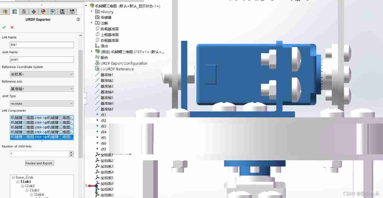
Detailed process of generating URDF file from SW model

STM32 project design: an e-reader making tutorial based on stm32f4
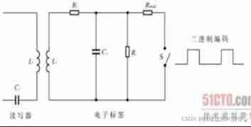
Fabrication of modulation and demodulation circuit

SOC wireless charging scheme

XXL job configuration alarm email notification

Whale conference provides digital upgrade scheme for the event site

鲸会务一站式智能会议系统帮助主办方实现数字化会议管理
随机推荐
torch. fft
Corn image segmentation count_ nanyangjx
Opencv learning notes 3
What is Qi certification Qi certification process
Leetcode: array fast and slow pointer method
GHUnit: Unit Testing Objective-C for the iPhone
optee中的timer代码导读
Fourier transform of image
Convert verification code image to tfrecord file
Assembly led on
ZLMediaKit推流拉流测试
STM32 project design: smart home system design based on stm32
Pandas vs. SQL 1_ nanyangjx
Golang JSON unsupported value: Nan processing
STM32 porting mpu6050/9250 DMP official library (motion_driver_6.12) modifying and porting DMP simple tutorial
STM32 project design: temperature, humidity and air quality alarm, sharing source code and PCB
Whale conference one-stop intelligent conference system helps organizers realize digital conference management
Transformers loading Roberta to implement sequence annotation task
Jupyter的安装
51 single chip microcomputer project design: schematic diagram of timed pet feeding system (LCD 1602, timed alarm clock, key timing) Protues, KEIL, DXP