当前位置:网站首页>Deep learning classification network -- alexnet
Deep learning classification network -- alexnet
2022-07-02 06:00:00 【occasionally.】
Deep learning classification network Summary
- AlexNet
- VGGNet
Catalog
- Deep learning classification network Summary
- Preface
- One 、 Network structure
- Two 、 Bright spot
- Reference material
- Pit to be filled ...
Preface
AlexNet By Hinton And its students Alex Designed by , To obtain the 2012 ILSVRC(ImageNet Large Scale Visual Recognition Challenge) The champion of the competition ,top5 Error rate for 15.3%, Far ahead of the second place 26.2%, The superiority of convolutional neural network in image recognition task is proved [1].
One 、 Network structure
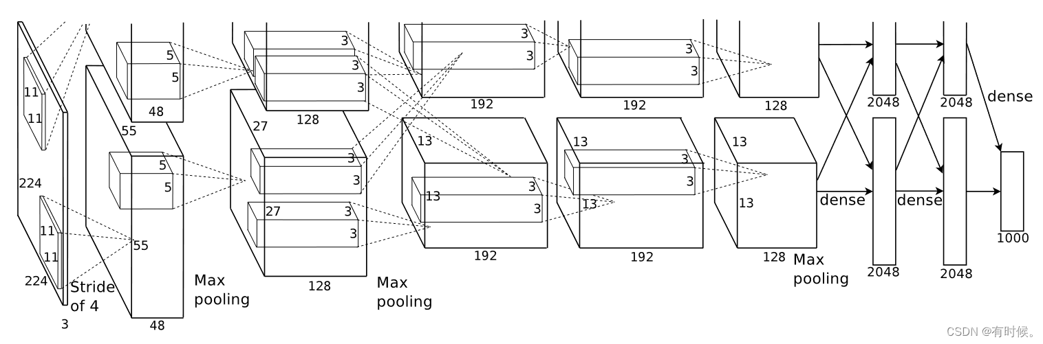
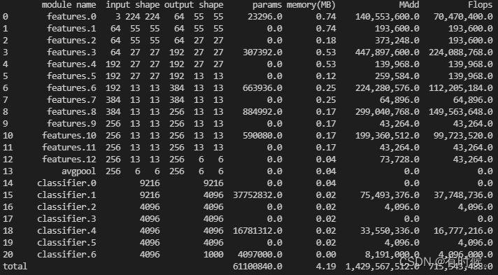
Quote the network structure diagram in the original paper , It can be seen that AlexNet share 8 layer ,5 Convolutions and 3 All connection layers . Use torchstat Tool printing pytorch Officially realized AlexNet Input and output dimensions of each layer in 、 Parameter quantity (parameters) And the amount of computation (FLOPs,MACs):
import torchvision.models as models
from torchstat import stat

alexnet = models.alexnet()
stat(alexnet, (3,224,224))

#  attach Pytorch Officially realized AlexNet structure , Different from the original paper
AlexNet(
  (features): Sequential(
    (0): Conv2d(3, 64, kernel_size=(11, 11), stride=(4, 4), padding=(2, 2))
    (1): ReLU(inplace=True)
    (2): MaxPool2d(kernel_size=3, stride=2, padding=0, dilation=1, ceil_mode=False)
    (3): Conv2d(64, 192, kernel_size=(5, 5), stride=(1, 1), padding=(2, 2))
    (4): ReLU(inplace=True)
    (5): MaxPool2d(kernel_size=3, stride=2, padding=0, dilation=1, ceil_mode=False)
    (6): Conv2d(192, 384, kernel_size=(3, 3), stride=(1, 1), padding=(1, 1))
    (7): ReLU(inplace=True)
    (8): Conv2d(384, 256, kernel_size=(3, 3), stride=(1, 1), padding=(1, 1))
    (9): ReLU(inplace=True)
    (10): Conv2d(256, 256, kernel_size=(3, 3), stride=(1, 1), padding=(1, 1))
    (11): ReLU(inplace=True)
    (12): MaxPool2d(kernel_size=3, stride=2, padding=0, dilation=1, ceil_mode=False)
  )
  (avgpool): AdaptiveAvgPool2d(output_size=(6, 6))
  (classifier): Sequential(
    (0): Dropout(p=0.5, inplace=False)
    (1): Linear(in_features=9216, out_features=4096, bias=True)
    (2): ReLU(inplace=True)
    (3): Dropout(p=0.5, inplace=False)
    (4): Linear(in_features=4096, out_features=4096, bias=True)
    (5): ReLU(inplace=True)
    (6): Linear(in_features=4096, out_features=1000, bias=True)
  )
)
Briefly summarize the input and output dimensions 、 Calculation method of parameter quantity and calculation quantity :
1. Input and output dimensions
The output size of convolution layer and pooling layer can be calculated according to the following formula : W o u t = W i n − K + 2 P S + 1 W_{out}=\frac{W_{in}-K+2P}{S}+1 Wout=SWin−K+2P+1 In the above formula : W i n W_{in} Win For input feature size ,K Is the convolution kernel size ,P by padding size , W o u t W_{out} Wout Is the dimension of the output characteristic drawing .
Take the first convolution layer for example : Input shape by (3,224,224), Convolution kernels for 11×11, In steps of 4,padding by (2,2), Parameters can be substituted : W o u t = 224 − 11 + 4 4 + 1 = 55.25 W_{out}=\frac{224-11+4}{4}+1=55.25 Wout=4224−11+4+1=55.25 Round down to 55, The number of convolution kernels is 64, So output shape by (64,55,55).
2. Parameter quantity
Convolution layer parameter quantity = ( K ∗ K ∗ C i n ) ∗ C o u t + C o u t (K*K*C_{in})*C_{out}+C_{out} (K∗K∗Cin)∗Cout+Cout, The full connection layer is regarded as K=1 Convolution layer of .
Take the first convolution layer for example :params = 11×11×3×64+64=23296
Take the first fully connected layer as an example :params = 1×1×9216×4096+4096=37752832
3. Amount of computation (FLOPs,MACs/MAdd)
- FLOPs(Float Point Operations): Number of floating point operations , Used to measure the complexity of an algorithm or model , Each plus 、 reduce 、 ride 、 Divide and calculate a floating-point operation .
- MACs(Multiply-Accumulate Operations): Multiply and add cumulative operation times , A multiply add accumulate operation includes a multiply operation and an add operation . therefore , There are usually FLOPs=2*MACs This relationship .
FLOPs computing method : Take convolution as an example , Suppose after convolution, output C o u t C_{out} Cout A dimension for H o u t × W o u t H_{out}×W_{out} Hout×Wout Characteristic graph , Each value in a single characteristic graph is calculated by convolution , So convoluted total FLOPs= H o u t × W o u t × C o u t H_{out}×W_{out}×C_{out} Hout×Wout×Cout × Convoluted FLOPs. A convolution calculation can be simplified to y = w x + b y=wx+b y=wx+b, there y y y Is to output a value in the characteristic graph , w w w by K × K × C i n K×K×C_{in} K×K×Cin The weight matrix of , w x wx wx contain K × K × C i n K×K×C_{in} K×K×Cin Multiplication operations and K × K × C i n − 1 K×K×C_{in}-1 K×K×Cin−1 An addition operation , + b +b +b contain 1 An addition operation , So the convolution is FLOPs= ( K × K × C i n ) + ( K × K × C i n − 1 ) + 1 = 2 ∗ K 2 ∗ C i n (K×K×C_{in})+(K×K×C_{in}-1)+1=2*K^2*C_{in} (K×K×Cin)+(K×K×Cin−1)+1=2∗K2∗Cin. So convoluted total FLOPs It can be calculated according to the following formula :
F L O P s ( c o n v ) = H o u t × W o u t × C o u t × 2 × K 2 × C i n ≈ 2 × p a r a m s × H o u t × W o u t FLOPs(conv) =H_{out}×W_{out}×C_{out}×2×K^2×C_{in} \approx2×params×H_{out}×W_{out} FLOPs(conv)=Hout×Wout×Cout×2×K2×Cin≈2×params×Hout×Wout(torchstat Medium FLOPs and MAdd It seems to be the reverse ?)
Two 、 Bright spot
1. ReLU Activation function
The author mentioned in his paper “ For the training time of gradient descent ,sigmoid and tanh Such a saturated nonlinear function is better than an unsaturated nonlinear function ReLU Much slower ”, The reason for the slow speed is sigmoid and tanh Function involves exponential operation , So in AlexNet Choose from ReLU Function as activation function .
#  Draw the active function image
import numpy as np
import matplotlib.pyplot as plt

plt.rc('font',family='Times New Roman', size=15)

x = np.linspace(-10,10,500)
sigmoid = 1 / (1+np.exp(-x))
tanh = (np.exp(x)-np.exp(-x)) / (np.exp(x)+np.exp(-x))
relu = np.where(x<0, 0, x)

fig = plt.figure()
ax = fig.add_subplot(211)
ax.spines['right'].set_visible(False)
ax.spines['top'].set_visible(False)
ax.spines['left'].set_position(('data',0))
ax.spines['bottom'].set_position(('data',0))
plt.plot(x, sigmoid, label='sigmoid')
plt.plot(x, tanh, label='tanh')
plt.grid(linestyle='-.')
plt.legend()
ax2 = fig.add_subplot(212)
ax2.spines['right'].set_visible(False)
ax2.spines['top'].set_visible(False)
ax2.spines['left'].set_position(('data',0))
ax2.spines['bottom'].set_position(('data',0))
plt.plot(x, relu, label='ReLU')
plt.grid(linestyle='-.')
plt.legend()
plt.tight_layout()
plt.show()

- The author proves through experiments that ReLU Compared to the function tanh The advantages of functions : Use ReLU Activate the four layers of the function CNN stay CIFAR-10 Reached on dataset 25% The speed ratio of error rate tanh The activation function is about fast 6 times .( The solid line in the figure below is ReLU, The dotted line is tanh)
- Except for the speed ,ReLU The activation function can also avoid the gradient disappearance problem caused by the saturation function .

2. GPU Parallel training
There is one mentioned in the paper GTX 580GPU Only 3GB Of memory , It limits the maximum size of the network that can be trained with it , So split the network into two GPU On , Two GOU You can directly read and write to each other's memory , Without going through the host memory , double gpu Network comparison gpu The network spends less training time . The parallelization scheme adopted by the author is to put half of the neurons in a single GPU On , Another technique is used :GPU Only communicate in a specific layer .
3. Local response normalization (LRN)
In neurobiology “ Lateral inhibition ” Concept ( An excited neuron can reduce the activity of surrounding neurons ) Inspired by the , The author proposed the local response normalization , The calculation method is as follows :
In style :
b x , y i b_{x,y}^{i} bx,yi It means the first one i i i Feature map in position ( x , y ) (x,y) (x,y) The value after local response normalization at
a x , y i a_{x,y}^{i} ax,yi It means the first one i i i Feature map in position ( x , y ) (x,y) (x,y) The value before local response normalization at
k , α , β k,\alpha, \beta k,α,β Is a super parameter
N N N Is the total number of characteristic graphs , n n n Indicates how many adjacent feature graphs are taken , Use them in position ( x , y ) (x,y) (x,y) Place the value of the ( That is, in the formula a x , y j a_{x,y}^{j} ax,yj) In sum
Pytorch There is one difference between the implementation method in and the original paper , take α \alpha α Change it to α n \frac{\alpha}{n} nα: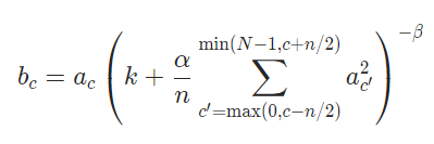
#  test Pytorch Medium LRN layer
import torch
import torch.nn as nn
import torch.nn.functional as F

lrn = nn.LocalResponseNorm(size=3, alpha=1, beta=1, k=1)
input_tensor = F.relu(torch.randn((1,4,3,3))) # (batchsize, C, H, W), 4 individual size by 3*3 Characteristic graph
output_tensor = lrn(input_tensor)

#  Before normalization
tensor([[[[0.0000, 0.0000, 0.0000],
          [1.5463, 1.2684, 1.5114],
          [0.6285, 1.6448, 0.0000]],

         [[0.5272, 0.0000, 0.3121],
          [0.9505, 0.0000, 0.0000],
          [0.0000, 0.0000, 0.0000]],

         [[1.1392, 0.0000, 0.0000],
          [0.0000, 0.0000, 0.0000],
          [0.1394, 0.0000, 0.5774]],

         [[1.0331, 1.0747, 0.0000],
          [1.0267, 0.9921, 0.0000],
          [0.0000, 0.0000, 0.0000]]]])
#  After normalization
tensor([[[[0.0000, 0.0000, 0.0000],
          [0.7370, 0.8256, 0.8580],
          [0.5554, 0.8649, 0.0000]],

         [[0.3457, 0.0000, 0.3023],
          [0.4530, 0.0000, 0.0000],
          [0.0000, 0.0000, 0.0000]],

         [[0.6056, 0.0000, 0.0000],
          [0.0000, 0.0000, 0.0000],
          [0.1385, 0.0000, 0.5197]],

         [[0.5777, 0.7760, 0.0000],
          [0.7598, 0.7470, 0.0000],
          [0.0000, 0.0000, 0.0000]]]])
Calculate it LRN Calculation process : Take the second characteristic graph in (0,0) Value at position 0.5272 For example , The lower limit of the summation channel is m a x ( 0 , 1 − 3 / 2 ) max(0,1-3/2) max(0,1−3/2)=0, Cap of m i n ( 4 − 1 , 1 + 3 / 2 ) = 2 min(4-1,1+3/2)=2 min(4−1,1+3/2)=2, So consider 0,1,2 Three channels , The substitution formula has :
b 0 , 0 1 = 0.5272 1 + ( 0 + 0.527 2 2 + 1.139 2 2 ) / 3 = 0.3457 b_{0,0}^1 = \frac{0.5272}{1+(0+0.5272^2+1.1392^2)/3}=0.3457 b0,01=1+(0+0.52722+1.13922)/30.5272=0.3457
4. Overlapping pooling
Use steps smaller than the size of the pooled window , Be able to obtain richer features ,top1 and top5 The error rates went down 0.4% and 0.3%.
5. Prevent over fitting
5.1 Data to enhance
- from 256×256 Crop immediately in the image 224×224, And translate and horizontally flip the cropped image . During the test TenCrop, Average 10 Picture of softmax Output as final output .
- change RGB Channel strength : Execute... On the image PCA, Then in each pixel of the original image (RGB Three channels ) Add the value calculated by the following formula
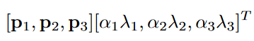
In the above formula : p i p_i pi and λ i \lambda_i λi For each RGB Pixel value of 3×3 Eigenvectors and eigenvalues of covariance matrix , p i p_i pi The dimensions are 3×1, Therefore, the calculation result of the above formula is 3×1, Three values are added to the pixel value RGB On three channels . α i \alpha_i αi Is subject to a mean of 0 And the standard deviation is 0.1 Gaussian variable of , Each training image is randomly generated once α i \alpha_i αi.
5.2 Dropout
Dropout technology : In each iteration of the neural network , With a certain probability p p p Randomly discard neurons , Make it not participate in forward and backward propagation in the current iteration .
- Integrating the prediction results of multiple models can effectively reduce the test error , But the cost of training multiple models is too high , Especially on large data sets .
- When... Is introduced into the network Dropout when , Each time new training data is received, a new network structure will be sampled , Train one subnet at a time , Multiple rounds of training is equivalent to integrating multiple sub networks . At testing time , All neurons are activated , But you need to multiply their output by the discard probability p p p.

6. Training strategy
6.1 SGD with momentum and weight decay
Small batch random gradient descent using large momentum and weight decay :batch size by 128, momentum by 0.9,weight decay by 0.0005.
6.2 Weight initialization
Proper weight initialization can speed up the learning of the network in the initial stage , In the text, all layers weights Initialize to w ∼ N ( 0 , 0.01 ) w\sim N(0,0.01) w∼N(0,0.01);bias Hierarchical initialization , second 、 Four 、 Five convolution layers and all fully connected layers bias Initialize to 1, Other layers are initialized to 0.
6.3 The learning rate has decreased
The initial learning rate of all layers is 0.01, When the error rate on the verification set no longer decreases, the learning rate decreases 1/10.
7. Convolution kernel Visualization
Reference material
[1] Krizhevsky A, Sutskever I, Hinton G E. ImageNet classification with deep convolutional neural networks[C]// International Conference on Neural Information Processing Systems. Curran Associates Inc. 2012:1097-1105.
[2] 【 Deep learning theory Convolutional neural networks 02】 General knowledge of convolution ( Calculate the shape of the output result according to the convolution kernel size and step size )
[3] CNN The computational power required for the model flops What is it? ? How to calculate ?
[4] 【 Local response normalization 】Local Response Normalization
[5] Srivastava N, Hinton G, Krizhevsky A, et al. Dropout: a simple way to prevent neural networks from overfitting[J]. The journal of machine learning research, 2014, 15(1): 1929-1958.
Pit to be filled …
- Summary of activation functions in Neural Networks
- Summary of normalization techniques in deep learning
- Summary of over fitting solutions
- Commonly used optimizers in deep learning
- Common weight initialization methods in neural networks
- Learning rate decay Strategy Summary
边栏推荐
- Go language web development is very simple: use templates to separate views from logic
- 【C语言】筛选法求素数
- 如何使用MITMPROXy
- Redis Key-Value数据库【初级】
- 文件包含漏洞(二)
- Unity Shader 学习笔记(3)URP渲染管线带阴影PBR-Shader模板(ASE优化版本)
- Eco express micro engine system has supported one click deployment to cloud hosting
- Unity shader learning notes (3) URP rendering pipeline shaded PBR shader template (ASE optimized version)
- [whether PHP has soap extensions installed] a common problem for PHP to implement soap proxy: how to handle class' SoapClient 'not found in PHP
- mysql的约束总结
猜你喜欢

深度学习分类网络--VGGNet

复杂 json数据 js前台解析 详细步骤《案例:一》

Stick to the big screen UI, finereport development diary
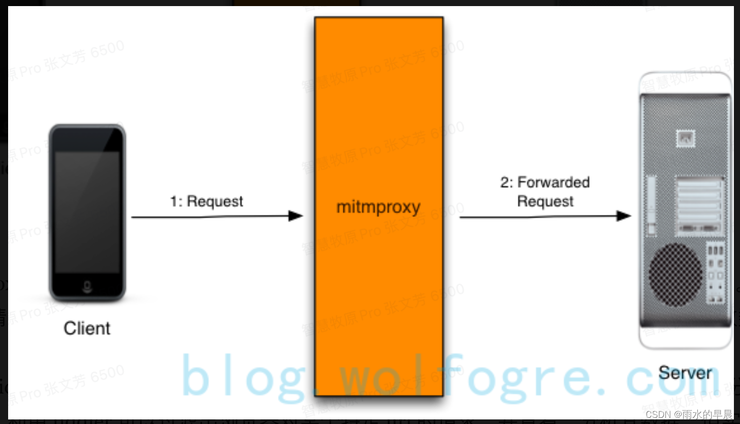
How to use mitmproxy
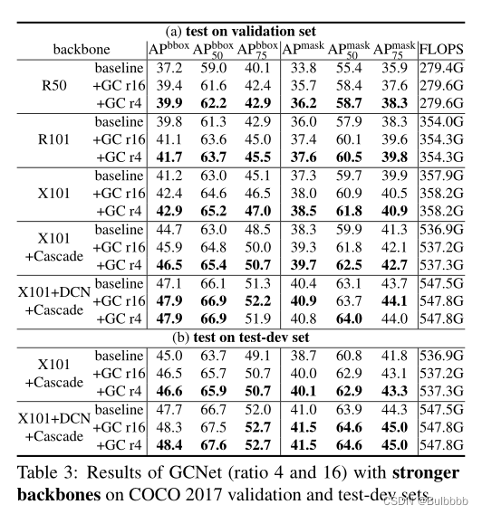
【論文翻譯】GCNet: Non-local Networks Meet Squeeze-Excitation Networks and Beyond
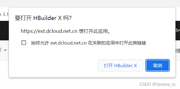
在uni-app中引入uView

Vscode paste image plugin saves image path settings

正则表达式总结
死磕大屏UI,FineReport开发日记

memcached安装
随机推荐
Stick to the big screen UI, finereport development diary
Fundamentals of software testing
1037 Magic Coupon
cookie插件和localForage离线储存插件
mysql的约束总结
php父类(parent)
servlet的web.xml配置详解(3.0)
Picture clipping plug-in cropper js
[C language] screening method for prime numbers
Verifying downloaded files using sha256 files
External interrupts cannot be accessed. Just delete the code and restore it Record this unexpected bug
php内类名称与类内方法名相同
我所理解的DRM显示框架
php按照指定字符,获取字符串中的部分值,并重组剩余字符串为新的数组
How to write good code - Defensive Programming Guide
php内的addChild()、addAttribute()函数
格式校验js
Zabbix Server trapper 命令注入漏洞 (CVE-2017-2824)
How vite is compatible with lower version browsers
Practice C language advanced address book design