Rewrite Boston house price forecast task (using paddlepaddlepaddle)

Rewrite the Boston house price forecast task （ Use a paddle paddlepaddle）

The Boston house price data set includes 506 Samples , Each sample includes 12 Two characteristic variables and the average house price in the area . housing price （ The unit price ） Obviously, it is related to multiple characteristic variables , Not univariate linear regression （ Univariate linear regression ） problem , Multiple characteristic variables are selected to establish the linear equation , This is multivariable linear regression （ Multiple linear regression ） problem . This paper discusses the use of propeller + Multiple linear regression , Solve the problem of housing price prediction in Boston .

1. Design of propeller “ Avenue ”

When we use the propeller framework to write multiple deep learning models , You will find that the program presents “ stereotyped writing ” The form of . That is, different programmers 、 Use different models 、 When solving different tasks , The modeling programs they write are very similar . Although these designs in some “ geek ” There is no brilliance in my eyes , But from a practical point of view , We expect the modeler to focus on the tasks that need to be solved , Instead of focusing on learning the framework . Therefore, there is a standard routine design for writing models with flying oars , Just master the method of using the propeller through an example program , It will be very easy to write multiple modeling programs for different tasks .

With this Python Our design ideas are consistent ： For a particular function , It's not that the more flexible the implementation 、 The more diverse, the better , It is better to have only one kind of conformity “ Avenue ” The best realization of . here “ Avenue ” It refers to how to better match people's thinking habits . When programmers first see Python Various application modes of , Feel that the program should be implemented naturally . But not all programming languages have such a combination “ Avenue ” The design of the , The design idea of many programming languages is that people need to understand the operating principle of machines , Instead of designing programs in the way humans are used to . meanwhile , Flexibility means complexity , It will increase the difficulty of communication between programmers , Nor is it suitable for the trend of modern industrialized production of software .

The original intention of the propeller design is not only to be easy to learn , Users are also expected to experience its beauty and philosophy , It is consistent with human's most natural cognition and usage habits .

2. Use the propeller to realize the Boston house price prediction task

The process of constructing neural network using propeller frame , Such as chart 1 Shown .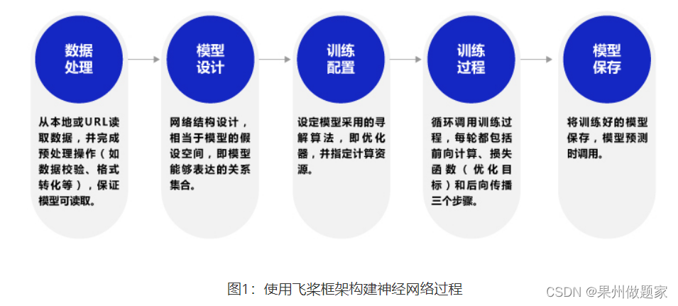

Before data processing , You need to load the relevant class libraries of the propeller framework first .

# Loading the propeller 、NumPy And related class libraries 
import paddle
from paddle.nn import Linear
import paddle.nn.functional as F
import numpy as np
import os
import random

The meaning of parameters in the code is as follows ：

• paddle： The main library of the propeller ,paddle Common... Are reserved in the root directory API Another name for , The present includes ：paddle.tensor、paddle.framework、paddle.device All under directory API;
• Linear： Full connection layer function of neural network , The basic neuron structure that contains the addition of all input weights . In the task of house price forecasting , Using a neural network with only one layer （ Fully connected layer ） Implement linear regression model .
• paddle.nn： Networking related API, Include Linear、 Convolution Conv2D、 Cyclic neural network LSTM、 Loss function CrossEntropyLoss、 Activation function ReLU etc. ;
• paddle.nn.functional： And paddle.nn equally , Including networking related API, Such as ：Linear、 Activation function ReLU etc. , Both contain modules with the same name and have the same functions , The operation performance is basically the same . The difference lies in paddle.nn All modules in the directory are classes , Each class has its own module parameters ;paddle.nn.functional All modules in the directory are functions , You need to manually pass in the parameters required by the function calculation . In actual use , Convolution 、 The full connection layer itself has learnable parameters , It is recommended to use paddle.nn; And the activation function 、 There are no learnable parameters for pooling and other operations , Consider using paddle.nn.functional.

---

explain ：

The propeller supports two deep learning modeling writing methods , The dynamic graph pattern which is more convenient for debugging and the static graph pattern which has better performance and is easy to deploy .

• Dynamic graph mode （ Imperative programming paradigm , analogy Python）： Analytical execution . Users do not need to define a complete network structure in advance , Write each line of network code , The calculation results can be obtained at the same time ;
• Static graph mode （ Declarative programming paradigm , analogy C++）： Compile first and then execute . Users need to define a complete network structure in advance , Then compile and optimize the network structure , To get the calculation results .

Propeller frame 2.0 And later , Dynamic graph mode is used for encoding by default , At the same time, it provides complete dynamic and static support , Developers only need to add a decorator （ to_static ）, The propeller will automatically convert the program of dynamic diagram into that of static diagram program, And use the program Train and save the static model to realize reasoning deployment .

---

2.1 Data processing

def load_data():
    #  Import data from file 
    datafile = 'housing.data'
    data = np.fromfile(datafile, sep=' ', dtype=np.float32)

    #  Each data includes 14 term , In front of it 13 Item is the influence factor , The first 14 Item is the corresponding median housing price 
    feature_names = [ 'CRIM', 'ZN', 'INDUS', 'CHAS', 'NOX', 'RM', 'AGE', \
                      'DIS', 'RAD', 'TAX', 'PTRATIO', 'B', 'LSTAT', 'MEDV' ]
    feature_num = len(feature_names)

    #  Take the raw data Reshape, become [N, 14] This shape 
    data = data.reshape([data.shape[0] // feature_num, feature_num])

    #  Split the original data set into training set and test set 
    #  Use here 80% Data for training ,20% Test the data 
    #  There must be no intersection between test set and training set 
    ratio = 0.8
    offset = int(data.shape[0] * ratio)
    training_data = data[:offset]

    #  Calculation train The maximum value of the data set , minimum value , Average 
    maximums, minimums, avgs = training_data.max(axis=0), training_data.min(axis=0), \
                                 training_data.sum(axis=0) / training_data.shape[0]
    
    #  Record the normalization parameters of the data , Normalize the data in the prediction 
    global max_values
    global min_values
    global avg_values
    max_values = maximums
    min_values = minimums
    avg_values = avgs

    #  Normalize the data 
    for i in range(feature_num):
        data[:, i] = (data[:, i] - avgs[i]) / (maximums[i] - minimums[i])

    #  The proportion of training set and test set 
    training_data = data[:offset]
    test_data = data[offset:]
    return training_data, test_data

#  Verify the correctness of the data set reader 
training_data, test_data = load_data()
print(training_data.shape)
print(training_data[1,:])

2.2 Model design

The essence of model definition is to define the network structure of linear regression , It is recommended to create Python Class to complete the definition of the model network , This class needs to inherit paddle.nn.Layer Parent class , And define... In the class init Functions and forward function .forward A function is a function specified by the framework to implement forward computing logic , The program will automatically execute when calling the model instance ,forward The network layer used in the function needs to be in init Function .

• Definition init function ： Declare the implementation function of each layer of network in the initialization function of the class . In the task of house price forecasting , Just define a layer of full connectivity ;
• Definition forward function ： Building neural network structure , Implement the forward computing process , And return the prediction results , In this task, we return the result of house price forecast .

class Regressor(paddle.nn.Layer):

    # self Represents the instance of the class itself 
    def __init__(self):
        #  Initialize some parameters in the parent class 
        super(Regressor, self).__init__()
        
        #  Define a layer of full connectivity , The input dimension is 13, The output dimension is 1
        self.fc = Linear(in_features=13, out_features=1)
    
    #  Forward computing of networks 
    def forward(self, inputs):
        x = self.fc(inputs)
        return x

2.3 Training configuration

The training configuration process is as follows: chart 2 Shown ：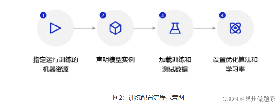

• Declare that the defined regression model instance is Regressor, And set the state of the model to train;
• Use load_data Function to load training data and test data ;
• Set optimization algorithm and learning rate , The optimization algorithm uses random gradient descent SGD, The learning rate is set to 0.01.

#  Declare a well-defined linear regression model 
model = Regressor()
#  Turn on the model training mode 
model.train()
#  Load data 
training_data, test_data = load_data()
#  Define optimization algorithms , Use random gradient descent SGD
#  The learning rate is set to 0.01
opt = paddle.optimizer.SGD(learning_rate=0.01, parameters=model.parameters())

---

explain ：

Model instances have two states ： Training state .train() And forecast status .eval(). Training to carry out forward calculation and back-propagation gradient two processes , The prediction only needs to perform the forward calculation , Specify the running state for the model , There are two reasons ：

1. Some high-level operators perform different logic in the two states , Such as ：Dropout and BatchNorm;
2. In terms of performance and storage space , More memory saving when predicting state ( There is no need to record the reverse gradient ), Better performance .

---

2.4 Training process

The training process adopts two-level circular nesting ：

• Inner circulation ： Responsible for one traversal of the entire data set , Batch by batch （batch）. Suppose the number of data set samples is 1000, A batch has 10 Samples , Then the number of batches traversing the dataset once is 1000/10=100, That is, the inner loop needs to execute 100 Time .

    for iter_id, mini_batch in enumerate(mini_batches):
  

• The outer loop ： Define the number of times to traverse the dataset , Through parameters EPOCH_NUM Set up .

    for epoch_id in range(EPOCH_NUM):
  

---

explain :

batch The value of will affect the training effect of the model ,batch Too big , It will increase memory consumption and computing time , And the training effect will not be significantly improved （ Each time the parameter moves only one small step in the opposite direction of the gradient , So the direction doesn't have to be particularly precise ）;batch Too small , Every batch The sample data has no statistical significance , The calculated gradient direction may deviate greatly . Because the training data set of house price prediction model is small , So it will batch Set to 10.

---

Each inner loop needs to be executed, such as chart 3 Steps shown , Calculation process and use Python The writing model is completely consistent .

• Data preparation ： Convert the data of a batch into nparray Format , To convert Tensor Format ;
• Forward calculation ： Pour the sample data of a batch into the network , Calculate the output ;
• Calculate the loss function ： Previously, the calculation results and real house prices were used as input , Through the loss function square_error_cost API Calculate the value of the loss function （Loss）.
• Back propagation ： Perform gradient back propagation backward function , That is, calculate the gradient of each layer from the back to the front , And update the parameters according to the set optimization algorithm (opt.step function ).

EPOCH_NUM = 10   #  Set the number of outer loops 
BATCH_SIZE = 10  #  Set up batch size 

#  Define the outer loop 
for epoch_id in range(EPOCH_NUM):
    #  Before each iteration begins , The sequence of training data is randomly disordered 
    np.random.shuffle(training_data)
    #  Split the training data , Every batch contain 10 Data 
    mini_batches = [training_data[k:k+BATCH_SIZE] for k in range(0, len(training_data), BATCH_SIZE)]
    #  Define the inner loop 
    for iter_id, mini_batch in enumerate(mini_batches):
        x = np.array(mini_batch[:, :-1]) #  Get the current batch training data 
        y = np.array(mini_batch[:, -1:]) #  Get the current batch training tag （ Real house price ）
        #  take numpy The data is converted to a propeller map tensor The format of 
        house_features = paddle.to_tensor(x)
        prices = paddle.to_tensor(y)
        
        #  Forward calculation 
        predicts = model(house_features)
        
        #  Calculate the loss 
        loss = F.square_error_cost(predicts, label=prices)
        avg_loss = paddle.mean(loss)
        if iter_id%20==0:
            print("epoch: {}, iter: {}, loss is: {}".format(epoch_id, iter_id, avg_loss.numpy()))
        
        #  Back propagation , Calculate the gradient value of each layer parameter 
        avg_loss.backward()
        #  Update parameters , Iterate one step according to the set learning rate 
        opt.step()
        #  Clear the gradient variable , For the next round of calculation 
        opt.clear_grad()

This implementation process is amazing , Forward calculation 、 Calculate the loss and back propagation gradient , Each operation only needs 1~2 One line of code ！ The propeller has helped us automatically realize the process of reverse gradient calculation and parameter update , There is no need to write code one by one , This is the power of using the propeller frame ！

2.5 Save and test the model

2.5.1 Save the model

Change the current parameter data of the model model.state_dict() Save to file , Program call for model prediction or verification .

#  Save model parameters , The file named LR_model.pdparams
paddle.save(model.state_dict(), 'LR_model.pdparams')
print(" The model was saved successfully , Model parameters are saved in LR_model.pdparams in ")

---

explain ：

Why do you want to save the model , Instead of directly using the trained model for prediction ？ In theory , The prediction can be completed by directly using the model instance , But in practice , Training model and usage model are often different scenarios . Model training usually uses a large number of offline servers （ No, customers of export-oriented enterprises / Users provide online services ）; Model prediction is usually realized by using the server that provides prediction services online, or embedding the completed prediction model into mobile phones or other terminal devices .

---

2.5.2 test model

Now select a data sample , Test the prediction effect of the model . The testing process is consistent with the process of using the model in the application scenario , It can be divided into the following three steps ：

1. Configure the machine resources predicted by the model . This case uses this machine by default , Therefore, there is no need to write code to specify .
2. Load the trained model parameters into the model instance . Completed by two statements , The first sentence is to read the model parameters from the file ; The second sentence is to load the parameter content into the model . After loading , You need to adjust the state of the model to eval()（ check ）. As mentioned above , The training state model needs to support both forward calculation and reverse conduction gradient , The implementation of the model is bloated , The model of checksum prediction state only needs to support forward calculation , The implementation of the model is simpler , Better performance .
3. Input the sample characteristics to be predicted into the model , Print out the prediction results .

adopt load_one_example Function to extract a sample from the data set as a test sample , The specific implementation code is as follows .

def load_one_example():
    #  From the test set loaded above , Randomly select one as the test data 
    idx = np.random.randint(0, test_data.shape[0])
    idx = -10
    one_data, label = test_data[idx, :-1], test_data[idx, -1]
    #  Modify this data shape by [1,13]
    one_data =  one_data.reshape([1,-1])

    return one_data, label

#  The parameter is the file address where the model parameters are saved 
model_dict = paddle.load('LR_model.pdparams')
model.load_dict(model_dict)
model.eval()

#  The parameter is the file address of the dataset 
one_data, label = load_one_example()
#  Turn data into dynamic graphs variable Format  
one_data = paddle.to_tensor(one_data)
predict = model(one_data)

#  Reverse normalizing the results 
predict = predict * (max_values[-1] - min_values[-1]) + avg_values[-1]
#  Yes label Inverse normalization of data 
label = label * (max_values[-1] - min_values[-1]) + avg_values[-1]

print("Inference result is {}, the corresponding label is {}".format(predict.numpy(), label))

By comparison “ Model predictions ” and “ Real house price ” so , The prediction effect of the model is close to the real house price . House price forecasting is only the simplest model , You can get twice the result with half the effort with flying oars . So for more complex models in industrial practice , The cost savings of using a propeller are immeasurable . At the same time, the performance of the propeller is optimized for many application scenarios and machine resources , In terms of function and performance, it is much stronger than the self written model .

3. Complete code

3.1 Data loading 、 Processing and model training

# Loading the propeller 、NumPy And related class libraries 
import paddle
from paddle.nn import Linear
import paddle.nn.functional as F
import numpy as np
import os
import random

def load_data():
    #  Import data from file 
    datafile = './work/housing.data'
    data = np.fromfile(datafile, sep=' ', dtype=np.float32)

    #  Each data includes 14 term , In front of it 13 Item is the influence factor , The first 14 Item is the corresponding median housing price 
    feature_names = [ 'CRIM', 'ZN', 'INDUS', 'CHAS', 'NOX', 'RM', 'AGE', \
                      'DIS', 'RAD', 'TAX', 'PTRATIO', 'B', 'LSTAT', 'MEDV' ]
    feature_num = len(feature_names)

    #  Take the raw data Reshape, become [N, 14] This shape 
    data = data.reshape([data.shape[0] // feature_num, feature_num])

    #  Split the original data set into training set and test set 
    #  Use here 80% Data for training ,20% Test the data 
    #  There must be no intersection between test set and training set 
    ratio = 0.8
    offset = int(data.shape[0] * ratio)
    training_data = data[:offset]

    #  Calculation train The maximum value of the data set , minimum value , Average 
    maximums, minimums, avgs = training_data.max(axis=0), training_data.min(axis=0), \
                                 training_data.sum(axis=0) / training_data.shape[0]
    
    #  Record the normalization parameters of the data , Normalize the data in the prediction 
    global max_values
    global min_values
    global avg_values
    max_values = maximums
    min_values = minimums
    avg_values = avgs

    #  Normalize the data 
    for i in range(feature_num):
        data[:, i] = (data[:, i] - avgs[i]) / (maximums[i] - minimums[i])

    #  The proportion of training set and test set 
    training_data = data[:offset]
    test_data = data[offset:]
    return training_data, test_data

class Regressor(paddle.nn.Layer):

    # self Represents the instance of the class itself 
    def __init__(self):
        #  Initialize some parameters in the parent class 
        super(Regressor, self).__init__()
        
        #  Define a layer of full connectivity , The input dimension is 13, The output dimension is 1
        self.fc = Linear(in_features=13, out_features=1)
    
    #  Forward computing of networks 
    def forward(self, inputs):
        x = self.fc(inputs)
        return x
    
#  Declare a well-defined linear regression model 
model = Regressor()
#  Turn on the model training mode 
model.train()
#  Load data 
training_data, test_data = load_data()
#  Define optimization algorithms , Use random gradient descent SGD
#  The learning rate is set to 0.01
opt = paddle.optimizer.SGD(learning_rate=0.01, parameters=model.parameters())

EPOCH_NUM = 10   #  Set the number of outer loops 
BATCH_SIZE = 10  #  Set up batch size 

#  Define the outer loop 
for epoch_id in range(EPOCH_NUM):
    #  Before each iteration begins , The sequence of training data is randomly disordered 
    np.random.shuffle(training_data)
    #  Split the training data , Every batch contain 10 Data 
    mini_batches = [training_data[k:k+BATCH_SIZE] for k in range(0, len(training_data), BATCH_SIZE)]
    #  Define the inner loop 
    for iter_id, mini_batch in enumerate(mini_batches):
        x = np.array(mini_batch[:, :-1]) #  Get the current batch training data 
        y = np.array(mini_batch[:, -1:]) #  Get the current batch training tag （ Real house price ）
        #  take numpy The data is converted to a propeller map tensor The format of 
        house_features = paddle.to_tensor(x)
        prices = paddle.to_tensor(y)
        
        #  Forward calculation 
        predicts = model(house_features)
        
        #  Calculate the loss 
        loss = F.square_error_cost(predicts, label=prices)
        avg_loss = paddle.mean(loss)
        if iter_id%20==0:
            print("epoch: {}, iter: {}, loss is: {}".format(epoch_id, iter_id, avg_loss.numpy()[0]))
        
        #  Back propagation , Calculate the gradient value of each layer parameter 
        avg_loss.backward()
        #  Update parameters , Iterate one step according to the set learning rate 
        opt.step()
        #  Clear the gradient variable , For the next round of calculation 
        opt.clear_grad()

#  Save model parameters , The file named LR_model.pdparams
paddle.save(model.state_dict(), 'LR_model.pdparams')
print(" The model was saved successfully , Model parameters are saved in LR_model.pdparams in ")

epoch: 0, iter: 0, loss is: 0.16621124744415283
epoch: 0, iter: 20, loss is: 0.14431345462799072
epoch: 0, iter: 40, loss is: 0.11563993990421295
epoch: 1, iter: 0, loss is: 0.13693055510520935
epoch: 1, iter: 20, loss is: 0.15183693170547485
epoch: 1, iter: 40, loss is: 0.2158908098936081
epoch: 2, iter: 0, loss is: 0.10545837879180908
epoch: 2, iter: 20, loss is: 0.058579862117767334
epoch: 2, iter: 40, loss is: 0.08427916467189789
epoch: 3, iter: 0, loss is: 0.06723933666944504
epoch: 3, iter: 20, loss is: 0.07996507734060287
epoch: 3, iter: 40, loss is: 0.026173889636993408
epoch: 4, iter: 0, loss is: 0.12865309417247772
epoch: 4, iter: 20, loss is: 0.1350513994693756
epoch: 4, iter: 40, loss is: 0.07391295582056046
epoch: 5, iter: 0, loss is: 0.16510571539402008
epoch: 5, iter: 20, loss is: 0.07523390650749207
epoch: 5, iter: 40, loss is: 0.03524921461939812
epoch: 6, iter: 0, loss is: 0.11212009191513062
epoch: 6, iter: 20, loss is: 0.033533357083797455
epoch: 6, iter: 40, loss is: 0.03091452643275261
epoch: 7, iter: 0, loss is: 0.03566620498895645
epoch: 7, iter: 20, loss is: 0.039590608328580856
epoch: 7, iter: 40, loss is: 0.07654304057359695
epoch: 8, iter: 0, loss is: 0.02911394275724888
epoch: 8, iter: 20, loss is: 0.021244537085294724
epoch: 8, iter: 40, loss is: 0.014933668076992035
epoch: 9, iter: 0, loss is: 0.06075896695256233
epoch: 9, iter: 20, loss is: 0.01793920248746872
epoch: 9, iter: 40, loss is: 0.014816784299910069
The model was saved successfully , Model parameters are saved in LR_model.pdparams in

3.2 Model test

# test model 
def load_one_example():
    #  From the test set loaded above , Randomly select one as the test data 
    idx = np.random.randint(0, test_data.shape[0])
    idx = -10
    one_data, label = test_data[idx, :-1], test_data[idx, -1]
    #  Modify this data shape by [1,13]
    one_data =  one_data.reshape([1,-1])

    return one_data, label

#  The parameter is the file address where the model parameters are saved 
model_dict = paddle.load('LR_model.pdparams')
model.load_dict(model_dict)
model.eval()

#  The parameter is the file address of the dataset 
one_data, label = load_one_example()
#  Turn data into dynamic graphs variable Format  
one_data = paddle.to_tensor(one_data)
predict = model(one_data)

#  Reverse normalizing the results 
predict = predict * (max_values[-1] - min_values[-1]) + avg_values[-1]
#  Yes label Inverse normalization of data 
label = label * (max_values[-1] - min_values[-1]) + avg_values[-1]

print("Inference result is {}, the corresponding label is {}".format(predict.numpy()[0,0], label))

Inference result is 26.6473445892334, the corresponding label is 19.700000762939453

3.3 Predicted results

import matplotlib.pyplot as plt
import warnings
%matplotlib inline
%config InlineBackend.figure_format = 'svg'

warnings.filterwarnings("ignore")

t = np.arange(len(label_1))
plt.rcParams['font.sans-serif'] = ['simHei']
plt.rcParams['axes.unicode_minus'] = False
plt.figure(facecolor='w',figsize=(8,4))
plt.plot(t, label_1, 'b-', lw=2, label=' True value ')
plt.plot(t, predict, 'r-', lw=2, label=' Estimated value ')
plt.legend(loc='best')
plt.title(' Boston house price forecast ', fontsize=18)
plt.xlabel(' Sample number ', fontsize=15)
plt.ylabel(' House price ', fontsize=15)
plt.grid()
plt.show()