当前位置：网站首页>Reinforcement learning - learning notes 2 | value learning

Reinforcement learning - learning notes 2 | value learning

2022-07-04 20:40:00 【climerecho】

Value-Based Reinforcement Learning : Value learning

2. Value learning

2.1 Deep Q-Network DQN

In fact, it is approximated by a neural network $Q*$ function .

agent Our goal is to win the game , If we use the language of reinforcement learning , Is the sum of the rewards you get at the end of the game Rewards The bigger the better .

a. Q-star Function

problem ： Suppose you know $Q^*(s,a)$ function , Which is the best action ？

obviously , The best action is $a^* = \mathop{argmax}\limits_{a}Q^*(s,a)$ ,

$Q^*(s,a)$ You can score each action , Like a prophet , Can tell you the average return of each action , Choose the action with the highest average return .

But the truth is , No one can predict the future , We don't know $Q^*(s,a)$. And value learning is to learn a function to approximate $Q^*(s,a)$ Make a decision .

solve ：Deep Q-network(DQN), That is, a neural network $Q(s,a;w)$ To approximate $Q^*(s,a)$ function .
The parameters of neural network are w , The input is the State s, Output is the scoring of all possible actions , Each action corresponds to a score .
Learn this neural network through rewards , This network will gradually improve the scoring of actions , More and more accurate
Play Super Mary millions of times , Can train a prophet .

b. Example

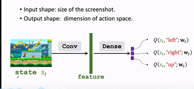
For different cases ,DQN The structure will be different .

If it's super Mary

Screen image as input
Use a convolution layer to turn the image into a feature vector
Finally, several fully connected layers are used to map the features to an output vector
The output vector is the score of the action , Each element of the vector corresponds to the score of an action ,agent Will choose the direction with the largest score to act .

c. use DQN Play the game

DQN The specific implementation process is as follows ：

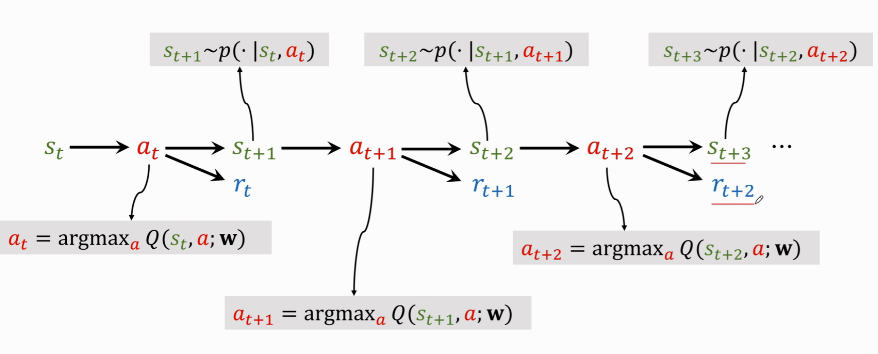
Step by step explanation ：

$ s_t \rightarrow a_t$： Current observed state $s_t$, Use formula $ a_t=\mathop{argmax}\limits_{a}Q^*(s,a)$ hold $s_t$ As input , Rate all actions , Choose the action with the highest score $a_t$ .
agent perform $a_t$ After this action , The environment will change the State , Use the state transition function $p(\cdot|s_t,a_t)$ Random sampling leads to a new state $s_{t+1}$.
The environment will also tell the rewards of this step $r_t$ , Reward is the supervisory signal in reinforcement learning ,DQN Train with these rewards .
With a new state $s_{t+1}$,DQN Continue to score all actions ,agent Choose the action with the highest score $a_{t+1}$.
perform $a_{t+1}$ after , The environment will update another status $s_{t+2}$, Give a reward $r_{t+1}$.
And then go back and forth , Until the end of the game

2.2 TD Study

How to train DQN ？ The most commonly used is Temporal Difference Learning.TD The principle of learning can be demonstrated by the following example ：

a. case analysis

Drive from New York to Atlanta , There's a model $Q(w)$ The predicted cost of driving is 1000 minute . This prediction may be inaccurate , More people are needed to provide data to train models to make predictions more accurate .

problem ： What kind of data is needed ？ How to update the model .

Let the model make a prediction before departure , Write it down as $q$,$q=Q(w)$, such as $q=1000$. Arrived at the destination , I found that only 860 minute , Get the real value $y=860$.
actual value $y$ And the forecast $q$ There is a deviation , That's what happened loss Loss
loss Defined as the actual value and the predicted value Square difference ：$L=\frac{1}{2}(q-y)^2$
On loss $L$ About parameters $w$ Take the derivative and expand it with the chain rule ：
$\frac{\partial L}{\partial w} = \frac{\partial q}{\partial w} \cdot \frac{\partial L}{\partial q} =(q-y)\cdot\frac{\partial Q(w)}{\partial w}$
The gradient is found , Gradient descent can be used to update model parameters w ：$w_{t+1} = w_t - \alpha \cdot \frac{\partial L}{\partial w} \vert _{w=w_t}$

shortcoming ： This algorithm is more naive, Because it takes the whole journey to complete an update of the model .

So here comes the question ： If you don't finish the whole trip , Whether the update of the model can be completed ？

It can be used TD Thinking about this matter . For example, we passed by halfway DC Don't go away , Didn't go to Atlanta , It can be used TD The algorithm completes the update of the model , namely

Pre departure forecast ：NYC -> Atlanta To spend 1000 minute , This is a Predictive value .
here we are DC when , It's found that 300 minute , This is a True observations , Although it is aimed at the part .
At this time, the model tells ,DC -> Atlanta To spend 600 minute .
The model originally predicted ：$Q(w) = 1000 $, And then DC New forecast ：300 + 600 = 900, This new 900 Valuation is called TD target .
Remember these nouns , It will be used repeatedly later ,TD target Is the use of the TD The moral overall prediction value of the algorithm .
TD target $y=900$ Although it is also an estimated forecast , But more than the original 1000 Minutes are more reliable , Because there are facts .
hold TD target $y$ Just As True value ：$L = \frac{1}{2}(Q(w)-y)^2$, among $Q(w) - y $ be called TD error.
Derivation ：$\frac{\partial L}{\partial w} =(1000-900)\cdot\frac{\partial Q(w)}{\partial w}$
Gradient descent updates model parameters w ：$w_{t+1} = w_t - \alpha \cdot \frac{\partial L}{\partial w} \vert _{w=w_t}$

b. Algorithm principle

Think about it from another angle ,TD This is the process of ：

Model to predict NYC -> Atlanta = 1000, DC -> Atlanta = 600, The difference between the two is 400, That is to say NYC -> DC = 400, But it only took 300 The difference between the estimated time in minutes and the real time is TD error：$\delta = 400-300 = 100$.

TD The goal of the algorithm is to make TD error As close as possible to 0 .

That is, we use part of the truth modify Part of the prediction , And make the overall prediction closer to reality . We can calibrate repeatedly The knowable part is true Come close to our ideal situation .

c. be used for DQN

(1) Formula introduction

There is such a formula in the above example ：$T_{NYC\rightarrow ATL} \approx T_{NYC\rightarrow DC} + T_{DC\rightarrow ATL} $

Want to use TD Algorithm , You have to use a formula like this , There is a term on the left side of the equation , There are two items on the right , One of them is actually observed .

And before that , There is also such a formula in deep reinforcement learning ：$Q(s_t,a_t;w)=r_t+\gamma \cdot Q(s_{t+1},a_{t+1};w)$.

Formula explanation ：
On the left is DQN stay t Estimates made at all times , This is the expectation of the sum of future rewards , amount to NYC To ATL Estimated total time .
On the right $r_t$ It is the reward of real observation , amount to NYC To DC .
$Q(s_{t+1},a_{t+1};w)$ yes DQN stay t+1 Estimates made at all times , amount to DC To ATL The estimated time .

(2) Formula derivation

Why is there such a formula ？

review Discounted return:$U_t=R_t+\gamma R_{t+1}+\gamma^2 R_{t+2}+\gamma^3 R_{t+3}+\cdots$
Put forward $\gamma$ You get $ = R_t + \gamma(R_{t+1}+ \gamma R_{t+2}+ \gamma^2 R_{t+3}+\cdots) $
The latter items can be written as $U_{t+1}$, namely $=R_t+\gamma U_{t+1}$
So you get ：$U_t = R_t + \gamma \cdot U_{t+1}$
Intuitively speaking , This is the mathematical relationship between two adjacent discount algorithms .

(3) Application process

Now we have to put TD The algorithm uses DQN On

t moment DQN Output value $Q(s_t,a_t; w)$ It's right $U_t$ Estimates made $\mathbb{E}[U_t]$, Be similar to NYC To ATL Estimated total time .
The next moment DQN Output value $Q(s_{t+1},a_{t+1}; w)$ It's right $U_{t+1}$ Estimates made $\mathbb{E}[U_{t+1}]$, Be similar to DC To ATL The second estimated time of .
because $U_t = R_t + \gamma \cdot U_{t+1}$
therefore $\underbrace{Q(s_t,a_t; w) }_{\approx\mathbb{E}[U_t]}\approx \mathbb{E}[R_t+\gamma \cdot \underbrace{Q(s_{t+1},a_{t+1}; w)}_{\approx\mathbb{E}[U_{t+1}]}]$
$\underbrace{Q(s_t,a_t;w)}_{prediction}=\underbrace{r_t+\gamma \cdot Q(s_{t+1},a_{t+1};w)}_{TD\ \ target}$

With prediction and TD target , You can update DQN The model parameters of .

t Time model makes predictions $Q(s_t,a_t;w_t)$;
here we are t+1 moment , Observed real rewards $r_t$ And the new state $s_{t+1}$, Then calculate the new action $a_{t+1}$.
At this time, we can calculate TD target Write it down as $y_t$, among $y_t=r_t+\gamma \cdot Q(s_{t+1},a_{t+1};w）$
t+1 The action of the moment $a_{t+1}$ How to calculate the ？DQN Score each action , Take the highest score , So it's equal to Q Function about a Maximize ：$ y_t = r_t + \gamma \cdot \mathop{max}\limits_{a} Q(s_{t+1},a;w_t）$
We want to predict $Q(s_{t},a_{t};w)$ As close as possible TD target $y_t$ , So we regard the difference between the two as Loss :
$L_t=\frac{1}{2}[Q(s_{t},a_{t};w)-y_t]^2$
Do gradient descent ：$w_{t+1} = w_t - \alpha \cdot \frac{\partial L}{\partial w} \vert _{w=w_t}$ Update model parameters w, To make the Loss smaller

2.3 summary

Value learning （ Ben is talking about DQN） Based on the optimal action value function Q-star ：
$Q^*(s_t,a_t) = \mathbb{E}[U_t|S_t=s_t,A_t=a_t]$
Yes $U_t$ Expect , Can score each action , Reflect the quality of each action , Use this function to control agent.
DQN Is to use a neural network $Q(s,a;w)$ To approximate $Q^*(s,a) $
1. The parameters of neural network are w , Input is agent The state of s
2. The output is for all possible actions $ a \in A$ Of
TD The algorithm process
1. Observe the current state $S_t = s_t $ And actions that have been performed $A_t = a_t$
2. use DQN Do a calculation , The input is the State $s_t$, Output is for action $a_t$ Of
  Write it down as $q_t$,$q_t = Q(s_t,a_t;w)$
3. Back propagation is right DQN Derivation ：$d_t = \frac{\partial Q(s_t,a_t;w)}{\partial w} |_{ w=w_t}$
4. Due to the execution of the action $a_t$, The environment will update to $s_{t+1}$, And give rewards $r_t$.
5. Find out TD target：$y_t = r_t + \gamma \cdot \mathop{max}\limits_{a} Q(s_{t+1},a_t;w）$
6. Do a gradient descent to update the parameters w , $w_{t+1} = w_t - \alpha \cdot (q_t-y_t) \cdot d_t$
7. Update the iteration ...