[point cloud processing paper crazy reading classic version 13] - adaptive graph revolutionary neural networks

Before reading this article , It should be understood that spectral graph convolution network

Abstract

• background ： Graph Convolutional Neural Networks (Graph CNNs) Can be regarded as generalized CNNs, Be able to effectively handle all kinds of graph data
• problem ： At present ,Graph CNNs Medium filters It's all based on Fixed or shared graph structure On , For actual data ,graph Structures differ in size and connectivity
• Method ： Propose a more generalized and flexible Graph CNNs, The network can transfer any graph Structure as input . In this way , Train for each graph Data learning task driven adaptation graph; In order to learn more efficiently graph, A distance metric learning
• Code ：TensorFlow edition

introduction

• In the point cloud classification task ,graph The topology of is more informative than point features
• At present Graph CNNs There are the following bottlenecks ：
  1. graph degree constraint
  2. It is required to keep the same input graph structure
  3. fixed graph
  4. Unable to learn topology information
• In this paper, a new spectral graph convolution network, In different ways graph Structure raw data as input . to batch Each individual sample in is assigned a specific graph Laplacian, Objectively describe its unique topology . specific graph Laplacian Will lead to specific spectral filter, according to graph Laplacian Distinctive graph Laplacian, spectral filter Be able to combine the characteristics of neighborhood .
• residual graph For exploring finer structural information
• a supervised metric learning with Mahalanobis distance Can reduce complexity
• Contributions：
  1. Construct unique graph Laplacian
  2. Learn distance metric for graph update
  3. Feature embedding in convolution
  4. Accept flexible graph inputs

Related work

The method referred to in this article will one-hop local kernel Extended to $K$-hop Connection . according to graph Fourier transform, If $U$ yes $L$ Of graph Fourier basis aggregate , that ：
$$x_{k+1}=\sigma \left(g_{\theta }\left(L^K\right)x_k\right)=\sigma \left(U{g}_{\theta }\left({\Lambda }^K\right)U^T{x}_k\right).$$
$\mathrm{diag}(\Lambda )$ yes $L$ Of frequency components.

Method

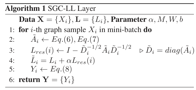
SGC-LL

Spectral Graph Convolution layer + Graph Laplacian Learning = SGC-LL

Learning Graph Laplacian

Given a graph $\mathcal{G}=(V,E)$, Its adjacency matrix is $A$, The degree matrix is $D$, Normalized Graph Laplacian matrix $L$ Expressed as ：
$$L=I-D^{-1/2}A{D}^{-1/2}$$
$L$ It represents the connectivity between nodes and the degree of vertices , got it $L$ It means you know $\mathcal{G}$ Topology of .

because $L$ Is a symmetric positive definite matrix , After its feature decomposition, a complete set of feature vectors will be obtained ${\left\{u_s\right\}}_{s=0}^{N-1}$ Composed of $U$,$N$ Represents the number of vertices . Use $U$ As graph Fourier basis,Graph Laplacian It can be diagonalized into $L=U\Lambda U^T$.

Graph Fourier Transformation is defined as $\hat{x}=U^{T}x$. because graph The spectrum of topological structure is expressed as $\Lambda$, So spectrum filter $g_{\theta }(\Lambda )$ Will generate a specific convolution in space kernel. By smooth frequency components Composed of spectrum Will form a local space kernel.$g_{\theta }(\Lambda )$ It can be expressed as a polynomial ：
$$g_{\theta }(\Lambda )=\sum _{k=0}^{K-1}{\theta }_k{\Lambda }^k,$$
This leads to a $K$-localized kernel, It allows any pair of shortest path distances $d_{\mathcal{G}}<K$ The summit of squeeze in.

Besides , Longer connections mean less similarity , And will be assigned by ${\theta }_k$ Less contribution of control . Polynomial filter smoothed spectrum, And by ${\theta }_k$ Parameterization also forces the final kernel From the central vertex to the farthest $K$-hop Circular weight distribution of vertices . That's the limit kernel The flexibility of the . what's more , The similarity between two vertices is essentially determined by the selected distance measurement and feature domain . For non Euclidean data , Euclidean distance is no longer guaranteed to be the best measure of similarity . therefore , Because the graph is suboptimal , Therefore, the similarity between connected nodes may be lower than that between disconnected nodes . There are also two possible reasons ：

• Graph It is constructed in the original feature domain before feature extraction and transformation
• The topology of a graph is intrinsic , It only represents the physical connection , For example, chemical bonds in molecules

In order to break the above restrictions , We propose a new spectral filter, Yes Laplacian $L$ Parameterize .

Given the original Laplacian $L$, features $X$ and Parameters $\Gamma$, function $\mathcal{F}(L,X,\Gamma )$ The output is updated Laplacian $\tilde{L}$ Of spectrum, that filter Will become ：
$$g_{\theta }(\Lambda )=\sum _{k=0}^{K-1}(\mathcal{F}(L,X,\Gamma ){)}^k$$
Final ,SGC-LL Layers can be represented as ：
$$Y=U{g}_{\theta }(\Lambda )U^{T}X=U\sum _{k=0}^{K-1}(\mathcal{F}(L,X,\Gamma ){)}^k{U}^{T}X.$$
Because it is dense matrix multiplication $U^{T}X$, So the complexity in the above formula is $\mathcal{O}\left(N^2\right)$. If $g_{\theta }(\tilde{L})$ It's through $\tilde{L}$ Polynomial function of recursive estimation , Then the complexity will be reduced to $\mathcal{O}(K)$, This is because Laplacian $\tilde{L}$ It's a sparse matrix . We choose Chebychev Expand the calculation $k$ Order polynomial $T_k(\tilde{L})X$.

Training Metric for Graph Update

about graph Structural data , Euclidean distance is not the best measure of vertex similarity , So this article uses $x_i$ and $x_j$ Between the Generalized Mahalanobis distance As a measure ：
$$\mathbb{D}\left(x_i,x_j\right)=\sqrt{{\left(x_i-x_j\right)}^{T}M\left(x_i-x_j\right)}.$$
If $M=I$, Then the above formula will degenerate into European distance . In this model , Positive semidefinite matrices $M=$$W_d{W}_d^T$, among $W_d$ yes SGCLL One of the training weights of layer . next , Use this distance to calculate Gauss kernel：
$${\mathbb{G}}_{x_i,x_j}=\exp \left(-\mathbb{D}\left(x_i,x_j\right)/\left(2{\sigma }^2\right)\right).$$
In the face of $\mathbb{G}$ After normalization , Get dense adjacency matrix $\hat{A}$.

Re-parameterization on feature transform

In the classic CNNs in , The output characteristics of convolution layer are obtained by adding all characteristic graphs , These characteristic maps are all through different filter Calculated independently . This means that the new feature depends not only on the adjacent vertex , There will be others intra-vertex The influence of characteristics .

however , stay graph convolution On , In the same graph It is impossible to create and train separate topologies for different vertex features . In order to construct intra-vertex and inter-vertex Mapping of features , We are SGC-LL Layer introduces a transformation matrix and an offset vector ：
$$Y=\left(U{g}_{\theta }(\Lambda )U^{T}X\right)W+b$$
In the $i$ layer , Transformation matrix $W_i\in {\mathbb{R}}^{d_{i-1}\times d_i}$ And offset $b_i\in {\mathbb{R}}^{d_i\times 1}$ And measurement $M_i$ Training together , among $d_i$ It's a feature dimension .

stay SGC-LL Layer , The parameters to be trained are $\left\{M_i,W_i,b_i\right\}$, The learning complexity is $\mathcal{O}\left(d_i{d}_{i-1}\right)$, No input graph The influence of size and degree , On the next floor SGC-LL in ,spectral filter Will be embedded in other feature fields , The metrics in this feature domain are different from other domains .

Residual Graph Laplacian

In molecular tasks , Because there is no prior knowledge about distance measurement , Measure $M$ Is initialized randomly , So it may take a long time to converge . In order to speed up training and improve the stability of learning graph topology , We put forward a reasonable assumption , That is, the optimal graph Laplacian $\hat{L}$ With primordial Laplacian $L$ There are small changes between ：
$$\hat{L}=L+\alpha L_{res}$$
let me put it another way , It's primitive Laplacian $L$ Has included a certain number of graph structural information , Some substructure information is not included , Some of them cannot be in intrinsic graph Virtual vertex connection for direct learning on . therefore , We don't study directly $\hat{L}$, It's learning residual graph Laplacian $L_{res}(i)=\mathcal{L}(M_i,X)$.$L_{res}(i)$ For the final graph The influence of topology is determined by $\alpha$ control ,SGC-LL Specific operations such as Algorithm 1 Shown .

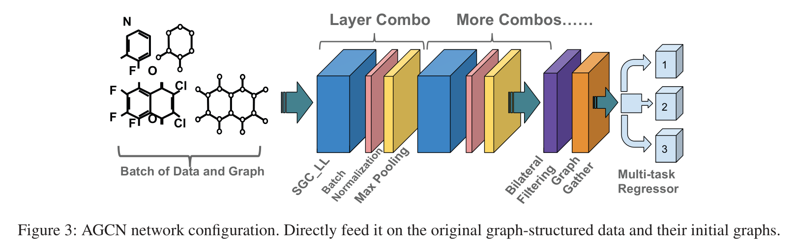
AGCN Network

AGCN Network = SGC-LL layer + graph max pooling layer + graph gather layer

Graph Max Pooling

Graph max pooling Between features . about graph Of the $v$ Features of vertices $x_v$, pooling The operation will change the $j$ Features $x_v(j)$, Replace with $j$ The largest of the four features , These features include adjacent vertices and themselves . If $N(v)$ yes $v$ A set of adjacent vertices , So at the top $v$ The new feature of is ：
$${\hat{x}}_v(j)=\max \left(\left\{x_v(j),x_i(j),\forall i\in N(v)\right\}\right)$$

Graph Gather

stay graph gather layer , Add all vertex eigenvectors , As graph Presentation of data .Gather layer The output of is used by vectors to predict . If not used graph gather layer , Then the network can be used for vertex prediction . Predictions in units of vertices include graph Complete and predict on social media .

Bilateral Filter

Bilateral filter layer The function of is to prevent over fitting ,residual graph Laplacian It will certainly adapt to the model to better fit the training task , But there is a risk of over fitting . In order to avoid over fitting , We introduce the modified bilateral filtering layer, By increasing $L$ The spatial locality of SGC-LL Regularize the activation result of . In addition to these , It's still used Batch normalization.

Network Configuration

layer combo = one SGC-LL layer + one batch normalization layer + one graph max pooling layer

Passing by a combo layer after ,batch Medium graph The structure has been updated , meanwhile grap The size remains the same .

Batch Training of Diverse Graphs

stay graph The biggest challenge of convolution on structured data is that it is difficult to match different local topologies of training samples .

Article SGC-LL layer Train individual Laplacian, All local topologies of the data structure are preserved . We found that , In the structure graph When the structure ,feature space and distance metrics It's very important ,SGC-LL layer Just need to batch All samples in share the same characteristic transformation matrix and distance metrics. Before training , You need to construct the initial graph Laplacians And according to these initial Laplacians to update kernel, This requires additional memory , But it's acceptable , because graph Laplacians Usually sparse .