[upsampling method opencv interpolation]

---

One 、 The introduction

interpolation (Interpolation), Usually refers to interpolation , It is a term of discrete mathematics , It is also an image processing term , The two are closely related . Zoom in and out as an image (Scale) The means of , Common traditional interpolation methods are ：

• Nearest neighbor interpolation (Nearest Neighbour Interpolation)
• linear interpolation (Linear Interpolation)
• Bilinear interpolation (Bilinear Interpolation)
• Bicubic interpolation (Bicubic interpolation)

wait , Even higher order linearity 、 Nonlinear interpolation method .

stay Discrete Mathematics in , Interpolation refers to the interpolation of continuous functions on the basis of discrete data , Make the continuous curve adopt
All given discrete data points . As an important method of discrete function approximation , By using interpolation, the value of the function at a finite number of points can be determined , Estimate the approximation of the function at other points .

This actually points out The essence of interpolation —— Use the known data to estimate the value of the unknown location . The image interpolation problem is similar to the fitting problem , Both of them are important parts of function approximation or numerical approximation . But the difference is ： For a given function , interpolation Discrete points are required “ Located in ” On the function curve to satisfy the constraint ; and fitting We hope that the discrete points can “ Close to ” Function curve .

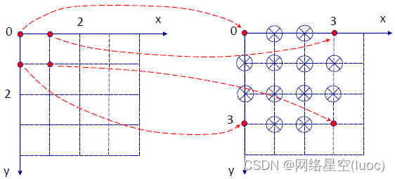
As for why we should interpolate , The figure above shows a two-dimensional image / Pixel coordinate system , Digital image magnification 3 Times local coordinate point transformation . For the coordinate points of the original image ( Red solid dot ), It's all on the new image Can determine one-to-one correspondence The coordinate point of ( Red solid dot ). As for the additional coordinate points in the new image due to enlargement ( Blue circle fork ), In the original image The corresponding point cannot be found 了 , What should I do ？ At this time , Interpolation technology came into being , Aimed at By certain rules / standard / constraint , Get the pixel values of these extra coordinate points . Take a simple one-dimensional example ：

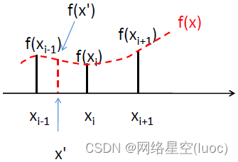
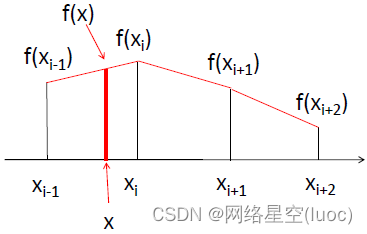
As shown in the figure above , Suppose that the coordinates of three discrete points on the number axis are xi-1,xi,xi+1. For a given continuous function f(x) As a constraint / The rules , The function values of the three-point coordinates are f(xi-1),f(xi), f(xi+1). At this time , If we want to get more dense 、 More subtle points , Then the coordinate value can be given , according to f(x) Get the function value . for example , set up xi-1 and xi A coordinate point between x’, according to f(x) Its function value is f(x’).

The above example is a simple one-dimensional interpolation representation ,f(x’) Is an interpolation result . in fact , Given different functional constraints f(x), We usually get different interpolation results , Therefore, there are many different interpolation methods , This article will illustrate these traditional linear interpolation principle .

Two 、 explain

2.1 Nearest neighbor interpolation (Nearest Neighbor Interpolation) —— Zero order interpolation

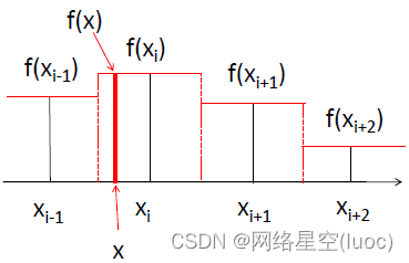
The figure above is a schematic diagram of one-dimensional nearest neighbor interpolation , Points on the coordinate axis xi-1,xi,xi+1 … Two halves equally spaced ( The red dotted line divides ), So each coordinate point of the non boundary has an equal width neighborhood , According to the value of each coordinate point, a function constraint similar to piecewise function is formed , Thus, the value of each interpolation coordinate point is equal to the value of the original coordinate point in the neighborhood . for example , Interpolation point x be seated Coordinates xi The neighborhood of , So its value f(x) Is equal to f(xi).

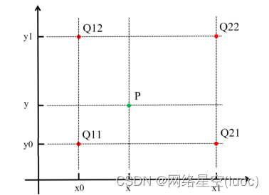
The above figure is a quantitative top view of two-dimensional nearest neighbor interpolation ,(x0, y0)、(x0, y1)、(x1, y0)、(x1, y1) Are all coordinate points on the original image , The gray values correspond to Q11、Q12、Q21、Q22. Interpolation points with unknown gray value (x, y), According to the constraints of the nearest neighbor interpolation method , It is related to the coordinate point (x0, y0) The position is closest to ( It is located in (x0, y0) In the neighborhood of ), Therefore, interpolation points (x, y) Gray value P = Q11.

Understand machine learning KNN (K - Nearest Neighbor) Algorithmic people will know , This is actually Equate to K=1 Of 1NN.

2.2 linear interpolation (Linear Interpolation) —— First order interpolation

The above figure is a qualitative diagram of one-dimensional linear interpolation , Points on the coordinate axis xi-1,xi,xi+1 … Value “ Two are directly connected ” For the line segment , Thus, a continuous constraint function is formed . Interpolation coordinate points, for example x, According to the constraint function, its value should be f(x). Because the constraint function curve between every two coordinate points is a linear line segment , For the interpolation result, it is “ linear ” Of , So this method is called linear interpolation .

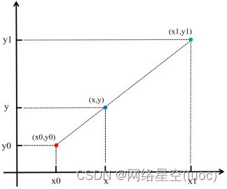
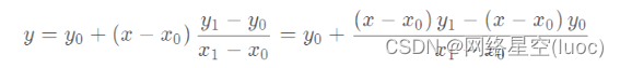
The figure above is a quantitative diagram of one-dimensional linear interpolation ,x0 and x1 Are the original coordinate points , The gray values correspond to y0 and y1. Interpolation points with unknown gray value x, Constraint according to linear interpolation method , stay (x0, y0) and (x1, y1) On the first-order function , Its gray value y That is to say ：

actually , Even if x be not in x0 And x1 Between , The formula also holds , But this method is called Linear extrapolation .

2.3 Bilinear interpolation (Bilinear Interpolation) —— First order interpolation

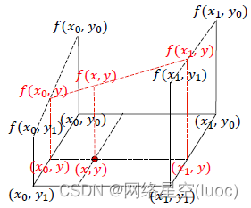
It is easy to expand from one-dimensional linear interpolation to two-dimensional image bilinear interpolation , Each time, the final result can be obtained through cubic first-order linear interpolation , The figure above shows a qualitative squint diagram of the process . among ,(x0, y0)、(x0, y1)、(x1, y0)、(x1, y1) Are the pixel coordinates on the original image , The gray values correspond to f(x0, y0)、f(x0, y1)、f(x1, y0)、f(x1, y1). Interpolation points with unknown gray value (x, y), According to the constraint of bilinear interpolation , You can start with the pixel coordinates (x0, y0) and (x0, y1) stay y One dimensional linear interpolation along the axis f(x0, y)、 By pixel coordinates (x1, y0) and (x1, y1) stay y One dimensional linear interpolation along the axis f(x1, y), And then by (x0, y) and (x1, y) stay x One dimensional linear interpolation is performed axially to obtain interpolation points (x, y) Gray value f(x, y). Of course , One dimensional linear interpolation is done first x Axial reworking y axial , The results are exactly the same , Just the difference of order , for example ：

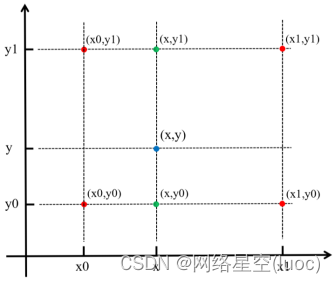
The above figure is a quantitative top view of two-dimensional bilinear interpolation ( The point position changes slightly but does not affect ), Let's change the order . Let's start with the pixel coordinates (x0, y0) and (x1, y0) stay x One dimensional linear interpolation along the axis f(x, y0)、 By pixel coordinates (x0, y1) and (x1, y1) stay x One dimensional linear interpolation along the axis f(x, y1)：

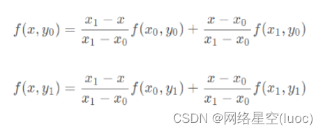
And then by (x, y0) and (x, y1) stay y One dimensional linear interpolation is performed axially to obtain interpolation points (x, y) Gray value f(x, y)：

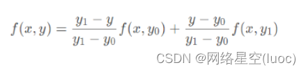
Merge the above formula , The final bilinear interpolation result is obtained ：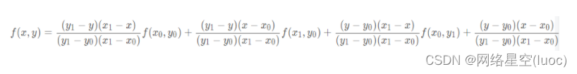

2.4 Bicubic interpolation (Bicubic Interpolation)

also called Cubic convolution interpolation / Bicubic interpolation , In numerical analysis , Bicubic interpolation is the most commonly used interpolation method in two-dimensional space . In this way , Interpolation point (x, y) Pixel gray value of f(x, y) Through a rectangular grid Weighted average of the last 16 sampling points obtain , and The weight of each sampling point is determined by the distance from the point to the interpolation point , This distance includes Horizontal and vertical The distance in both directions . by comparison , Bilinear interpolation is obtained by weighting the four surrounding sampling points .

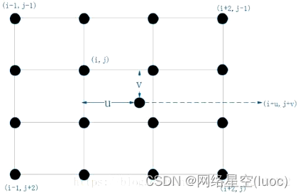
The above figure is a top view diagram of bicubic interpolation of a two-dimensional image . Let the coordinates of the interpolation points to be solved be (i+u, j+v), Know the surrounding 16 Pixel coordinates ( grid ) Gray value , You need to calculate 16 The weight of each point . In pixel coordinates (i, j) For example , Because the point is y Axis and x Axis direction and interpolation point to be solved (i+u, j+v) The distances are u and v, So the weight of is w(u) × w(v), among w(·) Is the interpolation weight kernel ( It can be understood as a defined weight function ). In the same way, you can get the rest 15 The weight of each pixel coordinate point . that , Interpolation points to be found (i+u, j+v) Gray value f(i+u, j+v) Will be calculated as follows ：

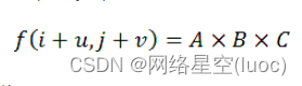
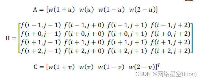
Where each term is represented by a vector or matrix as ：

Interpolation weight kernel w(·) by ：

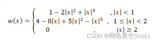
The function image is as follows ：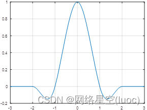

3、 ... and 、 Comparison and summary

Interpolation algorithm is often used for image scaling . The gray values of digital image pixels are discrete , Therefore, the general processing method is to interpolate the original pixel values on the integer point coordinates to generate a continuous surface , Then resample on the interpolation surface to obtain the gray value of the scaled image pixels . Zoom processing Start from the output image , use Reverse mapping Method , That is, find one or several pixels in the corresponding input image in the output image , This ensures that each pixel in the output image has a certain value . otherwise , If the output image is calculated from the input image , The pixels of the output image may have no gray value . Because when scaling the image , There may no longer be a one-to-one correspondence between the output image pixels and the input image . Practical application , Often use interpolation technology to increase graphic data , So that when printing or outputting in other forms , It can increase the printing area and ( or ) The resolution of the .

Nearest neighbor interpolation The advantage of this method is that the amount of calculation is very small , The algorithm is also simple , Therefore, the operation speed is faster . However, it only uses the gray value of the pixel closest to the sampling point to be measured as the gray value of the sampling point , Without considering the influence of other adjacent pixels , Therefore, there is obvious discontinuity in the gray value after resampling , The loss of image quality is large , Will produce obvious mosaic and sawtooth phenomenon .

Bilinear interpolation Method is better than nearest neighbor interpolation , Just a little more calculation , The algorithm is more complicated , The program runs a little longer , But after zooming, the image quality is high , It basically overcomes the discontinuity of nearest neighbor interpolation gray value , Because it takes into account the influence of the four direct neighboring points around the sampling point on the correlation of the sampling point . however , This method only considers the influence of the gray values of the four directly adjacent points around the sample point to be measured , Without considering the influence of the change rate of gray value between adjacent points , So it has the property of low-pass filter , This results in the loss of high-frequency components of the scaled image , The edge of the image becomes blurred to some extent . The output image scaled by this method is compared with the input image , There are still problems of image quality damage and low calculation accuracy due to poor consideration of interpolation function design .

Bicubic interpolation Method has the largest amount of calculation , The algorithm is also the most complex . In geometric operations , The smoothing effect of bilinear interpolation may degrade the details of the image , In the amplification process , The effect is more obvious . In other applications , The slope discontinuity of bilinear interpolation will produce undesirable results . Cubic convolution interpolation not only takes into account the influence of the gray values of the surrounding four directly adjacent pixels , The influence of the change rate of their gray values is also considered . Therefore, the shortcomings of the first two methods are overcome , It can produce smoother edges than bilinear interpolation , The calculation accuracy is very high , The image quality loss after processing is the least , The effect is the best .

All in all , When performing image scaling processing , The three algorithms should be selected according to the actual situation , We should consider the feasibility of time , The quality of the transformed image should also be considered , Only in this way can we achieve a more ideal Balance (trade-off).

Four 、 extend

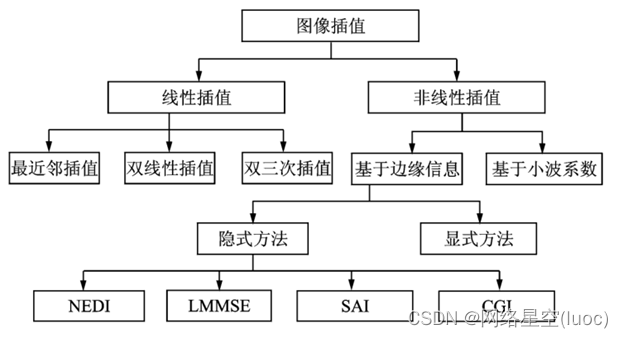
in fact , There are many interpolation techniques at present , As shown in the figure above , It can be roughly divided into two categories ： One is linear interpolation Method , Two is Nonlinear interpolation Method .

One side , The traditional interpolation methods are linear interpolation Method , Such as nearest neighbor interpolation 、 Bilinear interpolation 、 Bicubic interpolation, etc . This kind of method uses the same interpolation kernel in the interpolation process 、 There is no need to consider the position of the pixel to be inserted , So that the high-frequency part of the image —— The edge texture becomes blurred , Unable to achieve HD effect .

On the other hand , Nonlinear interpolation The main methods are ： be based on Wavelet coefficients Based on Edge information Methods . among , Methods based on edge information can be divided into Implicit methods and Explicit method . The implicit method contains ： Edge oriented interpolation (New edge directive interpolation,NEDI)、 Minimum mean square error estimation interpolation (Linear minimum mean square-error estimation,LMMSE)、 Soft decision adaptive interpolation (Soft-decision adaptive interpolation interpolation, SAI), Edge contrast guides image interpolation (Contrast-guided image interpolation, CGI) All of them are implicit interpolation methods based on image edges .

Besides , There are also later developments such as based on Decision tree 、 Dictionary learning 、 Deep learning And so on .

Code

1.resize（） Function definition

void resize(InputArray src, OutputArray dst, 
Size dsize, double fx=0, double fy=0, int interpolation=INTER_LINEAR)  

 Parameter description ：

src -  Original picture 

dst -  Target image . When parameters dsize Not for 0 when ,dst The size is size; otherwise , Its size depends on src Size , Parameters fx and fy decision .dst The type of （type） and src The image is the same 

dsize -  Target image size . When dsize by 0 when , It can be calculated by the following formula ：
dsize=Size(round(src.cols*fx),round(src.rows*fy))

 therefore , Parameters dsize And parameters (fx, fy) Can't be for at the same time 0

fx -  The scale factor on the horizontal axis . When it's for 0 when , The calculation formula is as follows ：

fy -  The scale factor on the vertical axis . When it's for 0 when , The calculation formula is as follows ：

interpolation -  Interpolation method . share 5 Kind of ：

１）INTER_NEAREST -  Nearest neighbor interpolation 

２）INTER_LINEAR -  Bilinear interpolation （ Default ）

３）INTER_AREA -  Resampling based on local pixels （resampling using pixel area relation）. For image extraction （image decimation） Come on , It might be a better way . But if it's zooming in , It's similar to the nearest neighbor method .

４）INTER_CUBIC -  be based on 4x4 Pixel neighborhood 3 Sub interpolation method 

５）INTER_LANCZOS4 -  be based on 8x8 Pixel neighborhood Lanczos interpolation 

2. matters needing attention

dsize and fx/fy You can't do it at the same time 0, Or you can specify dsize Value , Give Way fx and fy Vacancy directly uses the default value , Such as ：

1. resize(img, imgDst, Size(30,30)); Or set dsize by 0, Specify the good fx and fy Value , such as fx=fy=0.5, So it's equivalent to double the size of the original image in both directions ！

2. On the choice of interpolation methods , Normally, the default bilinear interpolation is used （INTER_LINEAR ） That's enough. . The efficiency of several common methods is ： Nearest neighbor interpolation > Bilinear interpolation > Bicubic interpolation >Lanczos interpolation ; But efficiency is inversely proportional to effectiveness , So use it according to your own situation .

3. Under normal circumstances , Before use dst The size and type of the image are unknown , Type from src Images are inherited , The size is also calculated from the original image according to the parameters . But if you've specified it in advance dst The size of the image , Then you can call the function in the following way ：resize(src, dst, dst.size(), 0, 0, interpolation);

3. Code example

#include <opencv2\opencv.hpp>
#include <opencv2\imgproc\imgproc.hpp>
 
using namespace cv;
 
int main()
{
    
	// Read image 
	Mat srcImage=imread("..\\1.jpg");
	Mat temImage,dstImage1,dstImage2;
	temImage=srcImage;
 
	// Show the original 
	imshow(" Original picture ",srcImage);
 
	// Size adjustment 
	resize(temImage,dstImage1,Size(temImage.cols/2,temImage.rows/2),0,0,INTER_LINEAR);
	resize(temImage,dstImage2,Size(temImage.cols*2,temImage.rows*2),0,0,INTER_LINEAR);
 
	imshow(" narrow ",dstImage1);
	imshow(" Zoom in ",dstImage2);
 
	waitKey();
	return 0;
 
}