当前位置:网站首页>Recommendation system (IX) PNN model (product based neural networks)
Recommendation system (IX) PNN model (product based neural networks)
2022-07-06 04:10:00 【Tianze 28】
Recommendation system ( Nine )PNN Model (Product-based Neural Networks)
Recommendation system series blog :
- Recommendation system ( One ) Overall overview of the recommendation system
- Recommendation system ( Two )GBDT+LR Model
- Recommendation system ( 3、 ... and )Factorization Machines(FM)
- Recommendation system ( Four )Field-aware Factorization Machines(FFM)
- Recommendation system ( 5、 ... and )wide&deep
- Recommendation system ( 6、 ... and )Deep & Cross Network(DCN)
- Recommendation system ( 7、 ... and )xDeepFM Model
- Recommendation system ( 8、 ... and )FNN Model (FM+MLP=FNN)
PNN Model (Product-based Neural Networks) And the last blog introduction FNN The model is the same , They are all from teacher Zhangweinan and his collaborators of Jiaotong University , This article paper Published in ICDM’2016 On , It's a CCF-B Class meeting , Personally, I have never heard of any company in the industry that has practiced this model in its own scenario , But we can still read this paper The results of , Maybe it can provide some reference for your business model . By the name of this model Product-based Neural Networks, We can also basically know PNN By introducing product( It can be inner product or outer product ) To achieve the purpose of feature intersection .
This blog will introduce motivation and model details .
One 、 motivation
This article paper The main improvement is introduced in the last blog FNN,FNN There are two main shortcomings :
- DNN Of embedding Layer quality is limited by FM The quality of training .
- stay FM Implicit vector dot product is used in feature intersection , hold FM Pre trained embedding The vector is sent to MLP Full link layer in ,MLP The full link layer of is essentially a linear weighted sum between features , That is to do 『add』 The operation of , This is related to FM A little inconsistent . in addition ,MLP Different field The difference between , All use linear weighted summation .
The original text of the paper is :
- the quality of embedding initialization is largely limited by the factorization machine.、
- More importantly, the “add” operations of the perceptron layer might not be useful to explore the interactions of categorical data in multiple fields. Previous work [1], [6] has shown that local dependencies between features from different fields can be effectively explored by feature vector “product” operations instead of “add” operations.
Actually, I think FNN There is also a big limitation :FNN It's a two-stage training model , It's not a data-driven Of end-to-end Model ,FNN There is still a strong shadow of traditional machine learning .
Two 、PNN Model details
2.1 PNN The overall structure of the model
PNN The network structure of is shown in the figure below ( The picture is taken from the original paper )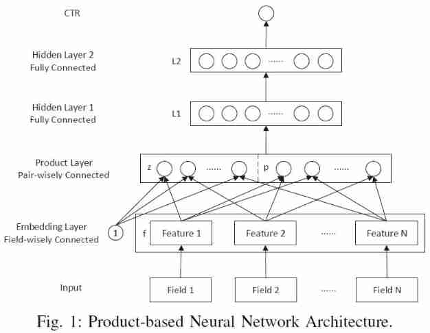
PNN The core of the model is product layer, It's the one in the picture above product layer pair-wisely connected This floor . But unfortunately , The picture given in the original paper hides the most important information , The first impression after reading the above picture is product layer from z z z and p p p form , Then send it directly to the upper L 1 L1 L1 layer . But it's not , What is described in the paper is : z z z and p p p stay product layer The transformation of the whole connection layer is carried out respectively , Separately z z z and p p p The mapping becomes D 1 D_1 D1 Dimension input vector l z l_z lz and l p l_p lp( D 1 D_1 D1 Is the number of neurons in the hidden layer ), And then l z l_z lz and l p l_p lp superposition , Then send it to L 1 L_1 L1 layer .
therefore , I will product layer Redraw , It looks more detailed PNN Model structure , As shown in the figure below :
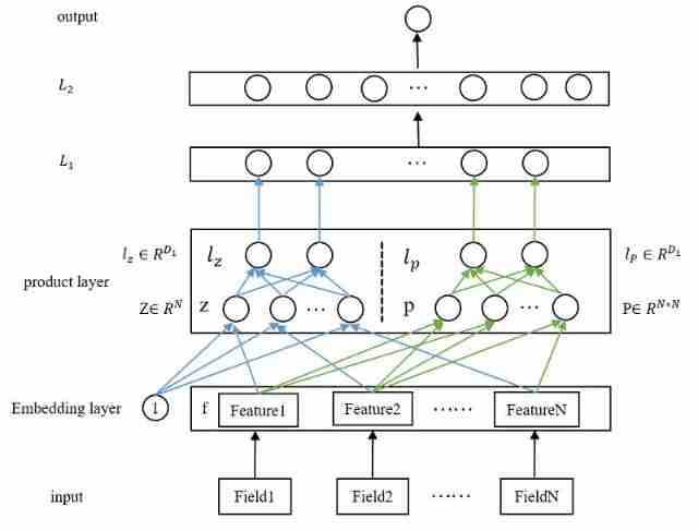
The above figure is basically very clear PNN The overall structure and core details of . Let's take a look at each floor from the bottom up
- Input layer
Original features , There's nothing to say . In the paper is N N N Features . - embedding layer
Nothing to say , Just an ordinary embedding layer , Dimension for D 1 D_1 D1. - product layer
The core of the whole paper , There are two parts here : z z z and p p p, Both are from embedding Layer .
【1. About z z z】
among z z z Is a linear signal vector , In fact, it's just to put N N N Characteristic embedding Vector directly copy To come over , A constant is used in the paper 1, Do multiplication . The paper gives a formal definition :
z = ( z 1 , z 2 , z 3 , . . . , z N ) ≜ ( f 1 , f 2 , f 3 , . . . , f N ) (1) z = (z_1,z_2,z_3,...,z_N) \triangleq (f_1,f_2,f_3,...,f_N) \tag{1} z=(z1,z2,z3,...,zN)≜(f1,f2,f3,...,fN)(1)
among ≜ \triangleq ≜ Is identity , therefore z z z The dimensions are N ∗ M N*M N∗M.
【2. About p p p】
p p p Here is the real cross operation , About how to generate p p p, The paper gives a formal definition : p i , j = g ( f i , f j ) p_{i,j}=g(f_i,f_j) pi,j=g(fi,fj), there g g g Theoretically, it can be any mapping function , This paper gives two kinds of mappings : The inner product and the outer product , Corresponding to IPNN and OPNN. therefore :
p = { p i , j } , i = 1 , 2 , . . . , N ; j = 1 , 2 , . . . , N (2) p=\{p_{i,j}\}, i=1,2,...,N;j=1,2,...,N \tag{2} p={ pi,j},i=1,2,...,N;j=1,2,...,N(2)
therefore , p p p The dimensions are N 2 ∗ M N^2*M N2∗M.
【3. About l z l_z lz】
With z z z after , Through a fully connected network , Such as in the figure above product layer in The blue line part , Finally mapped to D 1 D_1 D1 dimension ( Number of hidden layer units ) Vector , The formal expression is :
l z = ( l z 1 , l z 2 , . . . , l z k , . . . , l z D 1 ) l z k = W z k ⊙ z (3) l_z=(l_z^1,l_z^2,...,l_z^k,...,l_z^{D_1}) \ \ \ \ \ \ \ \ \ \ \ \ l_z^k=W_z^k\odot z \tag{3} lz=(lz1,lz2,...,lzk,...,lzD1) lzk=Wzk⊙z(3)
among , ⊙ \odot ⊙ Is the inner product symbol , Defined as : A ⊙ B ≜ ∑ i , j A i j A i j A\odot B\triangleq \sum_{i,j}A_{ij}A_{ij} A⊙B≜∑i,jAijAij, because z z z The dimensions are N ∗ M N*M N∗M, therefore W z k W_z^k Wzk The dimension of is also N ∗ M N*M N∗M.
【4. About l p l_p lp】
and l z l_z lz equally , Through a fully connected network , Such as in the figure above product layer in The green line , Finally mapped to D 1 D_1 D1 dimension ( Number of hidden layer units ) Vector , The formal expression is :
l p = ( l p 1 , l p 2 , . . . , l p k , . . . , l z D 1 ) l z k = W p k ⊙ p (4) l_p=(l_p^1,l_p^2,...,l_p^k,...,l_z^{D_1}) \ \ \ \ \ \ \ \ \ \ \ \ l_z^k=W_p^k\odot p \tag{4} lp=(lp1,lp2,...,lpk,...,lzD1) lzk=Wpk⊙p(4)
W p k W_p^k Wpk And p p p The dimensions of are the same , by N 2 ∗ M N^2*M N2∗M. - Fully connected layer
Here is the ordinary two-layer full connection layer , Go straight to the formula , Simple and clear .
l 1 = r e l u ( l z + l p + b 1 ) (5) l_1 = relu(l_z + l_p + b_1) \tag{5} l1=relu(lz+lp+b1)(5)
l 2 = r e l u ( W 2 l 1 + b 2 ) (6) l_2 = relu(W_2l_1 + b_2) \tag{6} l2=relu(W2l1+b2)(6) - Output layer
Because the scene is CTR forecast , So it is classified into two categories , Activate the function directly sigmoid,
y ^ = σ ( W 3 l 2 + b 3 ) (6) \hat{y} = \sigma(W_3l_2 + b_3) \tag{6} y^=σ(W3l2+b3)(6) - Loss function
Cross entropy goes ,
L ( y , y ^ ) = − y log y ^ − ( 1 − y ) log ( 1 − y ) ^ (7) L(y,\hat{y}) = -y\log\hat{y} - (1-y)\log\hat{(1-y)} \tag{7} L(y,y^)=−ylogy^−(1−y)log(1−y)^(7)
2.2 IPNN
stay product layer , On features embedding Vectors do cross , Theoretically, it can be any operation , This article paper Two ways are given : The inner product and the outer product , They correspond to each other IPNN and OPNN. In terms of complexity ,IPNN The complexity is lower than OPNN, Therefore, if you plan to implement the industry , Don't think about OPNN 了 , So I will introduce it in detail IPNN.
IPNN, That is to say product Layers do inner product operation , According to the definition of inner product given above , It can be seen that the result of the inner product of two vectors is a scalar . The formal expression is :
g ( f i , f j ) = < f i , f j > (8) g(f_i,f_j) = <f_i,f_j> \tag{8} g(fi,fj)=<fi,fj>(8)
Let's analyze IPNN Time complexity of , In defining the dimensions of the next few variables :embedding Dimension for M M M, The number of features is N N N, l p l_p lp and l z l_z lz The dimensions are D 1 D_1 D1. Because we need to cross the features in pairs , therefore p p p The size is N ∗ N N*N N∗N, So get p p p The time complexity of is N ∗ N ∗ M N*N*M N∗N∗M, With p p p, After mapping, we get l p l_p lp The time complexity of is N ∗ N ∗ D 1 N*N*D_1 N∗N∗D1, So for IPNN, Whole product The time complexity of the layer is O ( N ∗ N ( D 1 + M ) ) O(N*N(D1+M)) O(N∗N(D1+M)), This time complexity is very high , So it needs to be optimized , The technique of matrix decomposition is used in this paper , Reduce the time complexity to D 1 ∗ M ∗ N D1*M*N D1∗M∗N. Let's see how the paper is done :
Because the features intersect , therefore p p p It's obviously a N ∗ N N*N N∗N The symmetric matrix of , be W p k W_p^k Wpk It's also a N ∗ N N*N N∗N The symmetric matrix of , obviously W p k W_p^k Wpk It can be decomposed into two N N N Multiplied by dimensional vectors , hypothesis W p k = θ k ( θ k ) T W_p^k=\theta^k(\theta^k)^T Wpk=θk(θk)T, among θ k ∈ R N \theta^k\in R^N θk∈RN.
therefore , We have :
W p k ⊙ p = ∑ i = 1 N ∑ j = 1 N θ i k θ j k < f i , f j > = < ∑ i = 1 N θ i k f i , ∑ j = 1 N θ j k f j > (9) W_p^k \odot p = \sum_{i=1}^N\sum_{j=1}^N\theta^k_i\theta^k_j<f_i,f_j> = <\sum_{i=1}^N\theta^k_if_i, \sum_{j=1}^N\theta^k_jf_j> \tag{9} Wpk⊙p=i=1∑Nj=1∑Nθikθjk<fi,fj>=<i=1∑Nθikfi,j=1∑Nθjkfj>(9)
If we remember δ i k = θ i k f i \delta_i^k=\theta^k_if_i δik=θikfi, be δ i k ∈ R M \delta_i^k \in R^M δik∈RM, δ i k = ( δ 1 k , δ 2 k , . . . , δ N k ) ∈ R N ∗ M \delta_i^k=(\delta_1^k,\delta_2^k,...,\delta_N^k) \in R^{N*M} δik=(δ1k,δ2k,...,δNk)∈RN∗M.
therefore l p l_p lp by :
l p = ( ∣ ∣ ∑ i δ i 1 ∣ ∣ , . . . . , ∣ ∣ ∑ i δ i D 1 ∣ ∣ ) (10) l_p = (||\sum_i\delta_i^1||,....,||\sum_i\delta_i^{D_{1}}||) \tag{10} lp=(∣∣i∑δi1∣∣,....,∣∣i∑δiD1∣∣)(10)
The above series of formulas go up , It is estimated that there are not enough people interested in reading this blog 10% 了 , It's too obscure to understand . Want others to understand , The simplest way is to give examples , Let's go straight to the example , Suppose our sample has 3 Features , Every feature of embedding Dimension for 2, namely N = 3 , M = 2 N=3, M=2 N=3,M=2, So we have the following sample :
| features (field) | embedding vector |
|---|---|
| f 1 f_1 f1 | [1,2] |
| f 2 f_2 f2 | [3,4] |
| f 1 f_1 f1 | [5,6] |
It is represented by a matrix as :
[ 1 2 3 4 5 6 ] (11) \begin{bmatrix} 1& 2 \\ 3&4 \\ 5&6 \\ \end{bmatrix} \tag{11} ⎣⎡135246⎦⎤(11)
Then define W p 1 W_p^1 Wp1:
W p 1 = [ 1 2 3 2 4 6 3 6 9 ] (12) W_p^1 = \begin{bmatrix} 1& 2 & 3\\ 2&4 & 6\\ 3&6 &9 \\ \end{bmatrix} \tag{12} Wp1=⎣⎡123246369⎦⎤(12)
Let's separate them according to the ( The complexity is O ( N ∗ N ( D 1 + M ) ) O(N*N(D1+M)) O(N∗N(D1+M))) And decomposition, then calculate , As soon as we compare, we find the mystery .
- Before decomposition
Direct pair ( f 1 , f 2 , f 3 ) (f_1,f_2,f_3) (f1,f2,f3) Do the inner product in pairs to get the matrix p p p, The calculation process is as follows :
p = [ 1 2 3 4 5 6 ] ⋅ [ 1 3 5 2 4 6 ] = [ 5 11 17 11 25 39 17 39 61 ] (13) p = \begin{bmatrix} 1& 2 \\ 3&4 \\ 5&6 \\ \end{bmatrix} \cdot \begin{bmatrix} 1& 3 & 5 \\ 2&4 & 6 \\ \end{bmatrix} = \begin{bmatrix} 5& 11 & 17 \\ 11& 25 & 39 \\ 17& 39 & 61 \\ \end{bmatrix} \tag{13} p=⎣⎡135246⎦⎤⋅[123456]=⎣⎡51117112539173961⎦⎤(13)
among p i j = f i ⊙ f j p_{ij} = f_i \odot f_j pij=fi⊙fj.
With p p p, Let's calculate l p 1 l_p^1 lp1, In fact, it is an arithmetic 2 in product Layer l p l_p lp( The green part ) The value of the first element of , Yes :
W p 1 ⊙ p = [ 1 2 3 2 4 6 3 6 9 ] ⊙ [ 5 11 17 11 25 39 17 39 61 ] = s u m ( [ 5 22 51 22 100 234 51 234 549 ] ) = 1268 (14) W_p^1 \odot p = \begin{bmatrix} 1& 2 & 3\\ 2&4 & 6\\ 3&6 &9 \\ \end{bmatrix} \odot \begin{bmatrix} 5& 11 & 17 \\ 11& 25 & 39 \\ 17& 39 & 61 \\ \end{bmatrix} = sum(\begin{bmatrix} 5 &22 & 51 \\ 22 &100 &234 \\ 51 &234 &549 \\ \end{bmatrix}) = 1268 \tag{14} Wp1⊙p=⎣⎡123246369⎦⎤⊙⎣⎡51117112539173961⎦⎤=sum(⎣⎡522512210023451234549⎦⎤)=1268(14) - After decomposition
W p 1 W_p^1 Wp1 Obviously, it can be decomposed , Can be broken down into :
W p 1 = [ 1 2 3 2 4 6 3 6 9 ] = [ 1 2 3 ] [ 1 2 3 ] = θ 1 ( θ 1 ) T (15) W_p^1 = \begin{bmatrix} 1& 2 & 3\\ 2&4 & 6\\ 3&6 &9 \\ \end{bmatrix} = \begin{bmatrix} 1\\ 2\\ 3 \\ \end{bmatrix} \begin{bmatrix} 1&2&3\\ \end{bmatrix} = \theta^1 (\theta^1)^T \tag{15} Wp1=⎣⎡123246369⎦⎤=⎣⎡123⎦⎤[123]=θ1(θ1)T(15)
So according to the formula δ i 1 = θ i 1 f i \delta_i^1=\theta^1_if_i δi1=θi1fi, So let's calculate δ i 1 \delta_i^1 δi1, See the table below :
| features (field) | embedding vector | θ i 1 \theta^1_i θi1 | δ i 1 \delta_i^1 δi1 |
|---|---|---|---|
| f 1 f_1 f1 | [1,2] | 1 | [1,2] |
| f 2 f_2 f2 | [3,4] | 2 | [6,8] |
| f 1 f_1 f1 | [5,6] | 3 | [15,18] |
Because there is still a step to be done ∑ i = 1 N δ i 1 \sum_{i=1}^N\delta_i^1 ∑i=1Nδi1, therefore , Finally, we get the vector δ 1 \delta^1 δ1:
δ 1 = ∑ i = 1 N δ i 1 = [ 22 28 ] (16) \delta^1 = \sum_{i=1}^N\delta_i^1 = \begin{bmatrix} 22& 28 \end{bmatrix} \tag{16} δ1=i=1∑Nδi1=[2228](16)
So in the end :
< δ 1 , δ 1 > = δ 1 ⊙ δ 1 = [ 22 28 ] ⊙ [ 22 28 ] = 1268 (17) <\delta^1, \delta^1> = \delta^1 \odot \delta^1 = \begin{bmatrix} \tag{17} 22& 28 \end{bmatrix} \odot \begin{bmatrix} 22& 28 \end{bmatrix} = 1268 <δ1,δ1>=δ1⊙δ1=[2228]⊙[2228]=1268(17)
therefore , Finally we can find , Calculated before and after decomposition l p l_p lp The value of the first element of is the same , The time complexity after decomposition is only O ( D 1 ∗ M ∗ N ) O(D1*M*N) O(D1∗M∗N).
therefore , We are realizing IPNN When , The dimension of parameter matrix of linear part and cross part is :
- For linear weight matrix W z W_z Wz Come on , The size is D 1 ∗ N ∗ M D_1 * N * M D1∗N∗M.
- Pair crossover ( square ) Weight matrices W p W_p Wp Come on , The size is D 1 ∗ N D_1 * N D1∗N.
2.3 OPNN
OPNN and IPNN The only difference is that product layer Middle computation l p l_p lp From inner product to outer product , As a result of the outer product operation, we get a M ∗ M M*M M∗M Matrix , namely :
g ( f i , f j ) = f i f j T (18) g(f_i,f_j) = f_if_j^T \tag{18} g(fi,fj)=fifjT(18)
therefore ,OPNN The whole time is complicated as O ( D 1 M 2 N 2 ) O(D1M^2N^2) O(D1M2N2), The time complexity is also high , therefore , In this paper, a superposition (superposition) Methods , To reduce time complexity , Let's take a look at the formula :
p = ∑ i = 1 N ∑ j = 1 N f i f j T = f ∑ ( f ∑ ) T (19) p = \sum_{i=1}^N \sum_{j=1}^N f_i f_j^T = f_{\sum}(f_{\sum})^T \tag{19} p=i=1∑Nj=1∑NfifjT=f∑(f∑)T(19)
among , f ∑ = ∑ i = 1 N f i f_{\sum} = \sum_{i=1}^Nf_i f∑=∑i=1Nfi .
After the above simplification ,OPNN The time complexity is reduced to O ( D 1 M ( M + N ) ) O(D1M(M + N)) O(D1M(M+N)).
But let's look at the above formula (19), f ∑ = ∑ i = 1 N f i f_{\sum} = \sum_{i=1}^Nf_i f∑=∑i=1Nfi, This is equivalent to making an analysis of all features sum pooling, That is to add the corresponding dimension elements of different features , There may be some problems in the actual business , For example, two features : Age and gender , These two characteristics embedding Vectors are not in a vector space , Do this forcibly sum pooling May cause some unexpected problems . We pass only for multivalued features , For example, the user clicks in history item Of embedding Vector do pooling, There's no problem with that , because item Ben is in the same vector space , And it has practical significance .
In practice , I suggest to use IPNN.
reference
[1]: Yanru Qu et al. Product-Based Neural Networks for User Response Prediction. ICDM 2016: 1149-1154
边栏推荐
- 颠覆你的认知?get和post请求的本质
- [PSO] Based on PSO particle swarm optimization, matlab simulation of the calculation of the lowest transportation cost of goods at material points, including transportation costs, agent conversion cos
- Script lifecycle
- 如何修改表中的字段约束条件(类型,default, null等)
- Scalpel like analysis of JVM -- this article takes you to peek into the secrets of JVM
- Yyds dry goods inventory hcie security Day11: preliminary study of firewall dual machine hot standby and vgmp concepts
- Tips for using dm8huge table
- Stc8h development (XII): I2C drive AT24C08, at24c32 series EEPROM storage
- [adjustable delay network] development of FPGA based adjustable delay network system Verilog
- lora网关以太网传输
猜你喜欢
【PSO】基于PSO粒子群优化的物料点货物运输成本最低值计算matlab仿真,包括运输费用、代理人转换费用、运输方式转化费用和时间惩罚费用
关于进程、线程、协程、同步、异步、阻塞、非阻塞、并发、并行、串行的理解
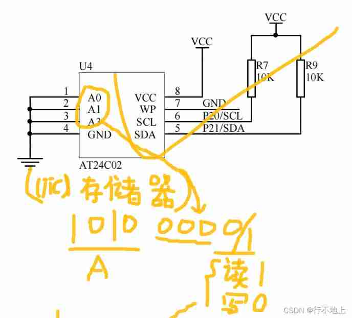
20、 EEPROM memory (AT24C02) (similar to AD)
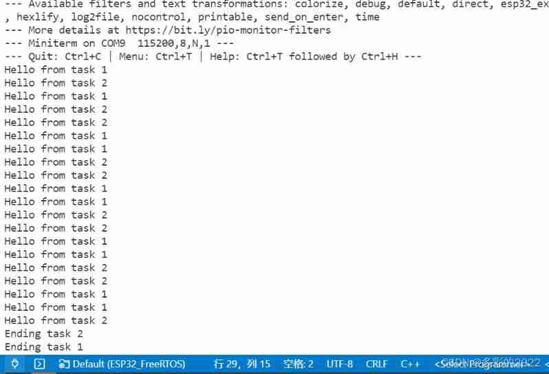
ESP32_ FreeRTOS_ Arduino_ 1_ Create task

C mouse event and keyboard event of C (XXVIII)
C (thirty) C combobox listview TreeView
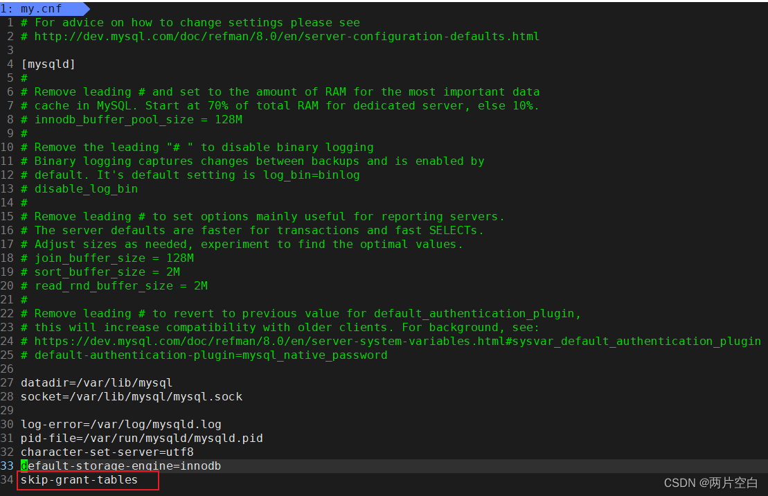
登录mysql输入密码时报错,ERROR 1045 (28000): Access denied for user ‘root‘@‘localhost‘ (using password: NO/YES
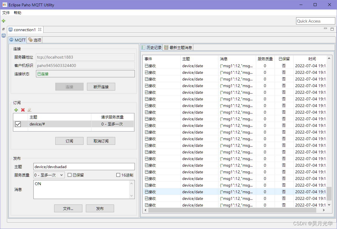
Esp32 (based on Arduino) connects the mqtt server of emqx to upload information and command control
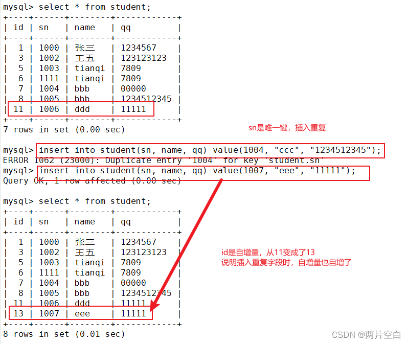
MySQL about self growth
10個 Istio 流量管理 最常用的例子,你知道幾個?
随机推荐
AcWing 243. A simple integer problem 2 (tree array interval modification interval query)
No qualifying bean of type ‘......‘ available
Benefits of automated testing
Leetcode32 longest valid bracket (dynamic programming difficult problem)
【可调延时网络】基于FPGA的可调延时网络系统verilog开发
Exchange bottles (graph theory + thinking)
Record the pit of NETCORE's memory surge
Codeforces Round #770 (Div. 2) B. Fortune Telling
STC8H开发(十二): I2C驱动AT24C08,AT24C32系列EEPROM存储
使用JS完成一个LRU缓存
[Zhao Yuqiang] deploy kubernetes cluster with binary package
Pandora IOT development board learning (HAL Library) - Experiment 9 PWM output experiment (learning notes)
[001] [stm32] how to download STM32 original factory data
MLAPI系列 - 04 - 网络变量和网络序列化【网络同步】
Explain in simple terms node template parsing error escape is not a function
P7735-[noi2021] heavy and heavy edges [tree chain dissection, line segment tree]
2/10 parallel search set +bfs+dfs+ shortest path +spfa queue optimization
KS008基于SSM的新闻发布系统
[Key shake elimination] development of key shake elimination module based on FPGA
2/13 review Backpack + monotonic queue variant