Hands on deep learning (III) -- convolutional neural network CNN

1 Image convolution

1.1 Cross correlation operation

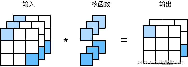
         stay ⼆ In dimensional cross-correlation operations , Convolution window from input ⼊ The upper left of tensor ⻆ Start , From left to right 、 Slide from top to bottom . When the convolution window slides to the new ⼀ Location (s) , The partial tensor contained in this window is related to the convolution kernel tensor ⾏ Multiply by elements , Then sum the tensors and get ⼀ A list ⼀ Scalar value of , From this we get this ⼀ Output tensor value of position . As shown in the figure below ：

         Be careful , Output ⼤ Little is less than losing ⼊⼤ Small . This is because the width of convolution kernel and ⾼ degree ⼤ On 1, The convolution kernel is only related to each ⼤ Small and completely suitable position ⾏ Cross correlation operation . therefore , Output ⼤ Less than equal to lose ⼊⼤ Small $n_h\times n_w$ Subtract the convolution kernel ⼤ Small $k_h\times k_w$, namely ：
$$(n_h-k_h+1)\times (n_w-k_w+1)$$

         This is because we need to ⾜ Enough space on the image “ Move ” Convolution kernel . later , We'll see how to fill in zeros around the image boundary to ensure that ⾜ Enough space to move the kernel , So as to maintain the output ⼤ Small unchanged . Next , We are corr2d Function to implement the above process , This function accepts input ⼊ tensor X And convolution kernel tensor K, And return the output tensor Y.

import torch 
def corr2d(X, K):
    """ Calculate two-dimensional cross-correlation operation """
    h, w = K.shape
    Y = torch.zeros((X.shape[0] - h +1, X.shape[1] - w +1))
    for i in range(Y.shape[0]):
        for j in range(Y.shape[1]):
            Y[i, j] = (X[i:i+h, j: j+w] * K).sum()
    return Y

         transport ⼊ tensor X And convolution kernel tensor K, To verify the above ⼆ Output of dimensional cross-correlation operation .

X = torch.tensor([[3, 3, 2, 1, 0], [0, 0, 1, 3, 1], [3, 1, 2, 2, 3], [2, 0, 0, 2, 2], [2, 0, 0, 0, 1]])
K = torch.tensor([[0, 1, 2], [2, 2, 0], [0, 1, 2]])
corr2d(X, K)        # tensor([[12., 12., 17.], [10., 17., 19.], [ 9., 6., 14.]])

1.2 Convolution layer

         Convolution layer transport ⼊ And convolution kernel weight ⾏ Cross correlation operation , And after adding scalar offset ⽣ Output . therefore , The two trained parameters in the convolution layer are convolution kernel weight and scalar offset . Just like before, we randomly initialize the full connection layer ⼀ sample , When training a convolution based model , We also initialize convolution kernel weights randomly .

         Based on ⾯ Defined corr2d Function implementation ⼆ Convolution layer . stay __init__ In the constructor , take weight and bias Declared as two model parameters . Forward propagation function modulation ⽤corr2d Function and add offset .

from torch import nn
class Conv2D(nn.Module):
    def __init__(self, kernel_size):
        super().__init__()
        self.weight = nn.Parameter(torch.rand(kernel_size))
        self.bias = nn.Parameter(torch.zeros(1))

    def forward(self ,x):
        return corr2d(x, self.weight) + self.bias

1.3 Edge detection of target in image

         The following is the convolution ⼀ A simple answer ⽤： By finding the location where the pixel changes , To detect different colors in the image ⾊ The edge of .⾸ First , We construct ⼀ individual $6\times 8$ Pixel ⿊⽩ Images . The middle four columns are ⿊⾊（0）, The rest of the pixels are ⽩⾊（1）.

X = torch.ones(6, 8)
X[:, 2:6] = 0

         Next , structure ⼀ individual ⾼ Degree is 1、 Width is 2 Convolution kernel K. When in ⾏ Cross correlation operation , If ⽔ The two adjacent elements are the same , The output is zero , Otherwise, the output is ⾮ zero .

K = torch.tensor([[1.0, -1.0]])

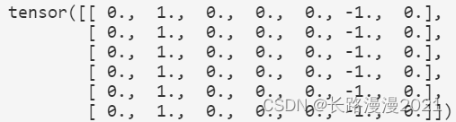
         Now? , We have parameters X（ transport ⼊） and K（ Convolution kernel ） Of board ⾏ Cross correlation operation . As follows ⽰, Output Y Medium 1 For from ⽩⾊ To ⿊⾊ The edge of ,-1 For from ⿊⾊ To ⽩⾊ The edge of , The output of other cases is 0.

Y = corr2d(X, K)
Y

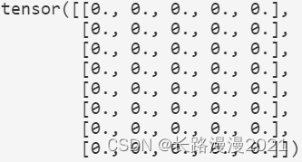
         Will lose ⼊ Of ⼆ Dimensional image transpose , Before going into ⾏ The above cross-correlation operation . Its output is as follows , The previously detected vertical edge disappears . It is as expected , This convolution kernel K Only vertical edges can be detected ,⽆ Method of detection ⽔ Flat edge .

corr2d(X.T, K)

2 Fill and stride

2.1 fill

         In response to ⽤ Multilayer convolution , We often lose edge pixels . Because we usually make ⽤ Small convolution kernel , So for any single convolution , We may only lose ⼏ Pixel . But as we should ⽤ Many continuous convolutions , The cumulative number of lost pixels is more . The simple way to solve this problem ⽅ Method is filling （padding）： Losing ⼊ The boundary filling elements of the image （ Usually the filling element is 0）. for example , In the following illustration , We will $3\times 3$ transport ⼊ Fill in $5\times 5$, Then its output will increase to $4\times 4$. The shaded part is the ⼀ Output elements and ⽤ Output of output calculation ⼊ And nuclear tensor elements ：$0\times 0+0\times 1+0\times 2+0\times 3=0$.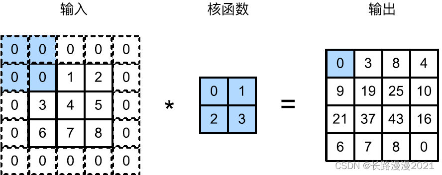

         Usually , If we add $p_h$⾏ fill （⼤ about ⼀ Half at the top ,⼀ Half at the bottom ） and $p_w$ Column fill （ left ⼤ about ⼀ And a half , On the right side ⼀ And a half ）, The output shape will be
$$(n_h-k_h+p_h+1)\times (n_w-k_w+p_w+1)$$

         This means that the output ⾼ Degree and width will be increased respectively $p_h$ and $p_w$.

         in many instances , We need to set $p_h=k_h-1$ and $p_w=k_w-1$, Lose ⼊ And output have the same ⾼ Degree and width . This allows you to build ⽹ It is easier to predict the output shape of each layer . hypothesis $k_h$ Is odd , We will be in ⾼ Fill both sides of degrees $p_h/2$⾏. If $k_h$ It's even , be ⼀ One possibility is to lose ⼊ Top filling $\lceil p_h/2\rceil$⾏, Fill the bottom with $\lfloor p_h/2\rfloor$⾏. Empathy , We fill both sides of the width .

         Convolution nerves ⽹ Convolution kernel in complex ⾼ Degrees and widths are usually odd , for example 1、3、5 or 7. The advantage of choosing odd numbers is , While maintaining the spatial dimension , We can fill the top and bottom with the same number of ⾏, Fill the left and right with the same number of columns .

import torch 
from torch import nn

def comp_conv2d(conv2d, X):
    """ This function initializes the volume layer weight , And lose ⼊ And output ⾼ And reduce the corresponding dimension """
    X = X.reshape((1, 1) + X.shape) #  this ⾥ Of （1,1） surface ⽰ Batch ⼤⼩ And the number of channels 1
    Y = conv2d(X)
    return Y.reshape(Y.shape[2:])   #  Omit the first two dimensions ： Batch ⼤⼩ And channel 

         establish ⼀ individual ⾼ Degree and width are 3 Of ⼆ Convolution layer , And fill all sides 1 Pixel . Given ⾼ Degree and width are 8 The loss of ⼊, The output of the ⾼ Degree and width are also 8.

conv2d = nn.Conv2d(1, 1, kernel_size=3, padding=1)  #  Each side is filled 1⾏ or 1 Column , A total of 2⾏ or 2 Column 
X = torch.rand(size=(8, 8))
comp_conv2d(conv2d, X).shape        # torch.Size([8, 8])

         When convolution kernel ⾼ Degree and width are different , We can fill in different ⾼ Degree and width , Make output and output ⼊ Have the same ⾼ Degree and width . In the following ⽰ In the example , We make ⽤⾼ Degree is 5, Width is 3 Convolution kernel ,⾼ The filling on both sides of degree and width are 2 and 1.

conv2d = nn.Conv2d(1, 1, kernel_size=(5, 3), padding=(2, 1))
comp_conv2d(conv2d, X).shape    # torch.Size([8, 8])

2.2 Stride

         Sometimes for ⾼ Efficient calculation or reducing the number of samples , The convolution window can skip the middle position , Slide multiple elements at a time .

         The number of elements per slide is called stride （stride）. To ⽬ The former is ⽌, We only make ⽤ too ⾼ Degree or width is 1 Stride , So how to make ⽤ a ⼤ The stride of ？ The following figure shows the vertical stride of 3,⽔ The flat stride is 2 Of ⼆ Dimensional cross correlation operation . the ⾊ Part is the output element and ⽤ Output of output calculation ⼊ And kernel tensor elements ：$0\times 0+0\times 1+1\times 2+2\times 3=8、0\times 0+6\times 1+0\times 2+0\times 3=6$.

The vertical stride is 3,⽔ The flat stride is 2 Of ⼆ Dimensional cross correlation operation

         Usually , When the vertical stride is $s_h$、⽔ The flat stride is $s_w$ when , The output shape is

$$\lfloor \left(n_h-k_h+p_h+s_h\right)/s_h\rfloor \times \lfloor \left(n_w-k_w+p_w+s_w\right)/s_w\rfloor$$

         Next ⾯ take ⾼ The strides of degree and width are set to 2, Thus will lose ⼊ Of ⾼ Half the degree and width .

conv2d = nn.Conv2d(1, 1, kernel_size=3, padding=1, stride=2)
comp_conv2d(conv2d, X).shape        # torch.Size([4, 4])

         When the convolution kernel size of height and width is different , When the filling and step size are different ,

conv2d = nn.Conv2d(1, 1, kernel_size=(3, 5), padding=(0, 1), stride=(3, 4))
comp_conv2d(conv2d, X).shape        # torch.Size([2, 2])

---

3 Multiple input multiple output channels

3.1 Multiple input channels

         When you lose ⼊ When multiple channels are included , It needs to be constructed ⼀ One and lose ⼊ Data has the same input ⼊ Convolution kernel of channel number , In order to lose ⼊ Data into ⾏ Cross correlation operation . Suppose you lose ⼊ The number of channels is $c_i$, So the input of convolution kernel ⼊ The number of channels also needs to be $c_i$. If the window shape of convolution kernel is $k_h\times k_w$, So when $c_i=1$ when , We can think of the convolution kernel as having the shape $k_h\times k_w$ Of ⼆ D tensor .

         However , When $c_i>1$ when , Each input of our convolution kernel ⼊ The channel will contain a shape of $k_h\times k_w$ Tensor . Put these tensors $c_i$ Link to ⼀ You can get a shape of $c_i\times k_h\times k_w$ Convolution kernel . Because of losing ⼊ And convolution kernel $c_i$ Channels , We can input for each channel ⼊ Of ⼆ Dimensional tensor and convolution kernel ⼆ Dimensional tensor into ⾏ Cross correlation operation , Then sum the channels （ take $c_i$ The results add up ） obtain ⼆ D tensor .

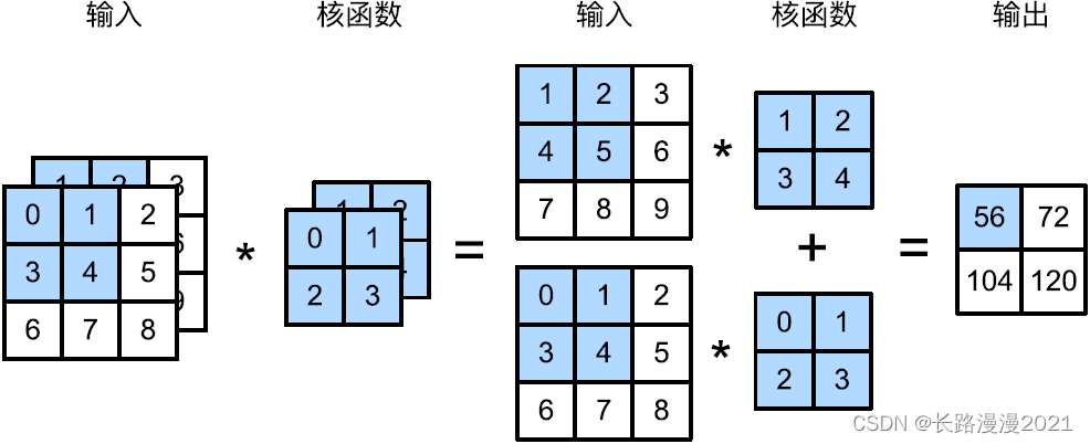
         The picture below shows ⽰ 了 ⼀ One has two losses ⼊ The tunnel ⼆ Dimensional cross-correlation operation ⽰ example . The shaded part is the ⼀ Output elements and ⽤ To calculate the output of this output ⼊ And nuclear tensor elements ：$(1\times 1+2\times 2+4\times 3+5\times 4)+(0\times 0+1\times 1+3\times 2+4\times 3)=56$.

Two lose ⼊ Cross correlation calculation of channels

         The following implementation ⼀ Lose more next ⼊ Channel cross correlation operation . Jane and ⾔ And , What we do is to hold on to each channel ⾏ Cross correlation operation , And then add up the results .

def corr2d_multi_in(X, K):
    """ First traversal “X” and “K” Of the 0 Dimensions （ Channel dimension ）, Add them to ⼀ rise """
    return sum(d2l.corr2d(x, k) for x, k in zip(X, K))

3.2 Multiple output channels

         At the top ⾏ The nerves of ⽹ Network structure , With the nerves ⽹ The deepening of the number of layers , We often increase the dimension of the output channel , By reducing the spatial resolution to obtain more ⼤ The depth of the passage . Intuitively speaking , We can think of each channel as a response to different characteristics . The reality may be more complicated ⼀ some , Because each channel is not unique ⽴ Study of the , But to work together ⽤ And optimized . therefore , Multiple output channels are not just detectors that learn multiple single channels .

        ⽤$c_i$ and $c_o$ Separate table ⽰ transport ⼊ And the number of output channels ⽬, And let $k_h$ and $k_w$ Is a convolution kernel ⾼ Degree and width . In order to obtain the output of multiple channels , We can create for each output channel ⼀ The shape is $c_i\times k_h\times k_w$ Convolution kernel tensor , So the shape of the convolution kernel is $c_o\times c_i\times k_h\times k_w$. In cross-correlation operation , Each output channel obtains all outputs first ⼊ passageway , Then the convolution kernel corresponding to the output channel is used to calculate the result .

         As follows ⽰, We implement ⼀ A cross-correlation function that calculates the output of multiple channels .

def corr2d_multi_in_out(X, K):
    #  iteration “K” Of the 0 Dimensions , Lose every time ⼊“X” Of board ⾏ Cross correlation operation 
    #  Finally, add all the results together 
    return torch.stack([corr2d_multi_in(X, k) for k in K], 0)

3.3 1×1 Convolution layer

         send ⽤ The smallest Window ,$1\times 1$ Convolution loses the unique energy of convolution ⼒—— stay ⾼ Degree and width dimensions , Identify the interaction between adjacent elements ⽤ Yes ⼒. Actually $1\times 1$ Convolution only ⼀ Calculate and send ⽣ On the aisle .

         Show below ⽰ Made ⽤$1\times 1$ Convolution kernel and 3 A loss ⼊ Channels and 2 Cross correlation calculation of two output channels . this ⾥ transport ⼊ And output have the same ⾼ Degree and width , Every element in the output is a slave ⼊ Same in image ⼀ Linear combination of elements of position . We can $1\times 1$ The convolution layer is seen as the position of each pixel should ⽤ The full connection layer of , With $c_i$ A loss ⼊ Value to co The output values . Because it's still ⼀ Convolution layers , So the weight across pixels is ⼀ To . meanwhile ,$1\times 1$ The weight dimension required by the convolution layer is $c_o\times c_i$, Plus ⼀ A deviation .

Cross correlation calculation makes ⽤ Has 3 A loss ⼊ Channels and 2 Of two output channels 1×1 Convolution kernel . among , transport ⼊ And output have the same ⾼ Degree and width

         Next ⾯, We make ⽤ Full connection layer implementation $1\times 1$ Convolution . Please note that , We need to lose ⼊ And the output data shape ⾏ fine-tuning .

def corr2d_multi_in_out_1(X, K):
    c_i, h, w = X.shape
    c_o = K.shape[0]
    X = X.reshape(c_i, h * w)
    K = K.reshape(c_o, c_i)
    #  Matrix multiplication in fully connected layers 
    Y = torch.matmul(K, X)
    return Y.reshape(c_o, h, w)

---

4 Convergence layer

4.1 Maximum convergence layer and average convergence layer

         Similar to convolution , The convergence layer operator consists of ⼀ A fixed shaped window , The window depends on its stride ⼤ Small is losing ⼊ Slide on all areas of , Fixed shape window （ Sometimes called convergence window ） Each position traversed is calculated ⼀ Outputs . However , Different from the transport in the convolution ⼊ Cross correlation calculation with convolution kernel , The aggregation layer does not contain parameters . contrary , The pool operator is deterministic , We usually calculate the most ⼤ Value or average . These operations are called the most ⼤ Convergence layer （maximum pooling） And the average convergence layer （average pooling）.

The shape of the convergence window is 22 The most ⼤ Convergence layer

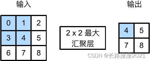
         In both cases , And the cross-correlation operator ⼀ sample , Convergence window from input ⼊ The upper left of tensor ⻆ Start , From left to right 、 Losing from top to bottom ⼊ Tensor slip . At every location reached by the convergence window , It calculates the input in the window ⼊⼦ Tensor's most ⼤ Value or average . Calculate the most ⼤ The value or average depends on making ⽤ Most ⼤ Convergence layer or average convergence layer .

         Under ⾯ In the code of pool2d function , Realize forward propagation of convergence layer . This function is similar to that in the previous section corr2d function . However , this ⾥ We have no convolution kernel , Output is output ⼊ The most ⼤ Value or average .

def pool2d(X, pool_size, mode='max'):
    p_h, p_w = pool_size
    Y = torch.zeros(X.shape[0] - p_h + 1, X.shape[1] - p_w + 1)
    for i in range(Y.shape[0]):
        for j in range(Y.shape[1]):
            if mode == 'max':
                Y[i, j] = X[i: i + p_h, j : j + p_w].max()
            elif mode == 'avg':
                Y[i, j] = X[i: i+p_h, j : j + p_w].mean()
    return Y

4.2 Fill and stride

         By default , Step length and convergence window in the deep learning framework ⼤ Little same . therefore , If we make ⽤ Shape is (3, 3) The convergence window , So by default , The step shape we get is (3, 3).

pool2d = nn.MaxPool2d((2, 3), padding= (0, 1), stride=(2, 3))

4.3 Multiple channels

         Dealing with multi-channel transmission ⼊ Data time , The convergence layer is at each transmission ⼊ Separate operation on the channel , Not like a convolution ⼀ The sample is matched on the channel ⼊ Into the ⾏ Summary . This means that the number of output channels in the convergence layer is related to the output ⼊ Same number of channels .