[differential privacy and data adaptability] differential privacy code implementation series (XIV)

Let me write it out front

When books come to school, they feel shallow , We must know that we must do it .

review

1、 The local model also has an obvious disadvantage ： Under the central differential privacy , For the same privacy cost as the same query , The accuracy of query results in local models is usually several orders of magnitude lower . This huge loss of accuracy means that only a few query types are suitable for local differential privacy , Even for these query types , It also requires a large number of participants .

2、 When the answer itself is small , The error of the local model will increase . In error , The random response is several orders of magnitude worse than the Laplace mechanism in the central model . Even if the local model has better algorithms , However, the inherent limitation of adding noise before submitting data means that the accuracy of the local model algorithm is always worse than that of the best central model algorithm .

3、 Other methods for performing histogram queries in local models have been proposed , Including some methods detailed in the previous paper . These can improve the accuracy to a certain extent , However, in the local model, the basic limitation of differential privacy of each sample must be ensured, which means , Even the most complex technologies cannot match the accuracy of the mechanisms we see in the central model .

Synthetic data

The importance of data for privacy protection is self-evident , What kind of data can use differential privacy , How to use it has become one of the key problems .

In this post , The problem of generating synthetic data using differential privacy algorithm will be studied . Strictly speaking , The input of this algorithm is the original data set , Its output has the same shape （ That is, the same number of columns and rows ） Synthetic data set .

Besides , We want the values in the composite dataset to have the same properties as the corresponding values in the original dataset .

for example , If we use the U.S. census data set as raw data , Then we hope that our synthetic data has a participant age distribution similar to the original data , And preserve the correlation between columns （ for example , The connection between age and occupation ）.

Most algorithms used to generate such synthetic data rely on the synthetic representation of the original data set , This representation does not have the same shape as the original data , But it is allowed to answer queries about raw data .

for example , If we only care about queries in different age ranges , Then we can generate an age histogram - How many participants in the raw data have each possible age - And use histograms to answer queries .

This histogram is a composite representation , It is suitable for answering some queries , But its shape is different from the original data , So it's not synthetic data .

Some algorithms only use synthetic representations to answer queries . Others use synthetic representations to generate synthetic data . We will introduce a synthetic representation , Histogram and several methods of generating synthetic data from it .

Histogram

We have seen many histograms , They are the main content of differential privacy analysis , Because it can be applied immediately In parallel . We also saw the concept of range query , Although we don't often use the name .

As the first step to obtain synthetic data , We will design a composite representation for a column of the original data set , This column can answer the range query .

Range query calculates the number of rows in the dataset with values within a given range . for example ," How many participants are aged 21 To the age of 33 Between the ages of ？" It's a range query .

def range_query(df, col, a, b):
    return len(df[(df[col] >= a) & (adult[col] < b)])

range_query(adult, 'Age', 21, 33)

We can define a histogram query , The query is 0 To 100 Between each age define a histogram bar , And use range query to calculate the number of people in each column .

The result looks very similar to calling plt.hist Data output , Because we basically calculate the same result manually .

bins = list(range(0, 100))
counts = [range_query(adult, 'Age', b, b+1) for b in bins]
plt.xlabel('Age')
plt.ylabel('Number of Occurrences')
plt.bar(bins, counts);

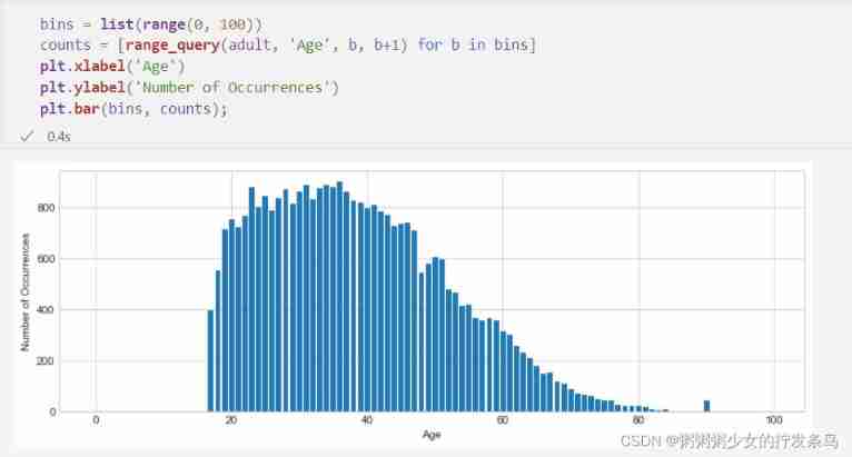
We can use these histogram results as a synthetic representation of the original data ！ To answer the range query , We can add up all the counts of the bars in this range .

def range_query_synth(syn_rep, a, b):
    total = 0
    for i in range(a, b):
        total += syn_rep[i]
    return total
    
range_query_synth(counts, 21, 33)

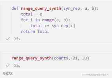
Please note that , Whether we issue range queries on raw data or synthetic representations , We will all get exactly the same result . We have not lost any information in the original data set （ At least for the purpose of answering the age range query ）.

Add differential privacy

We can easily make our synthetic data satisfy differential privacy . We can add Laplacian noise to each count in the histogram , Through parallel combination , It's satisfying $ϵ$- Differential privacy .

epsilon = 1
dp_syn_rep = [laplace_mech(c, 1, epsilon) for c in counts]

We can use the same function as before , Use our differential privacy composite representation to answer range queries .

Through post-processing , These results also meet $ϵ$- Differential privacy .

Besides , Because we rely on post-processing , So we can answer any number of queries as needed , Without additional privacy costs .

range_query_synth(dp_syn_rep, 21, 33)

How accurate the result is ？ For small areas , The results we get from the synthetic representation are similar to those obtained by Laplace The mechanism is directly applied to the results of the range query we want to answer, and the results can be obtained with very similar accuracy . for example ：

true_answer = range_query(adult, 'Age', 30, 31)
print('Synthetic representation error: {}'.format(pct_error(true_answer, range_query_synth(dp_syn_rep, 30, 31))))
print('Laplace mechanism error: {}'.format(pct_error(true_answer, laplace_mech(true_answer, 1, epsilon))))

As the scope grows , The larger the count , Therefore, we expect the error to improve .

We have seen this again and again , Larger groups mean stronger signals , This leads to a lower relative error .

Through the Laplace mechanism , We just saw this behavior . However , Through our synthetic representation , We add together the noise results from many smaller groups . So as the signal grows , Noise will also increase ！

therefore , Regardless of the size of the range , When we use composite representation, we will see roughly the same relative error size , Contrary to the Laplace mechanism ！

true_answer = range_query(adult, 'Age', 30, 71)
print('Synthetic representation error: {}'.format(pct_error(true_answer, range_query_synth(dp_syn_rep, 30, 71))))
print('Laplace mechanism error: {}'.format(pct_error(true_answer, laplace_mech(true_answer, 1, epsilon))))

This difference proves the shortcomings of our synthetic representation ： It can answer any range query it covers , But it may not be able to provide with Laplace Same accuracy of mechanism .

The main advantage of our synthetic representation is Be able to answer unlimited queries without extra privacy budget , The main drawback is the loss of accuracy .

Generate table data

The next step is from our synthetic representation to synthetic data .

So , We want to treat the composite representation as a probability distribution , The probability distribution estimates the basic distribution from which the original data is obtained , And take samples . Because we Consider only one column , Ignore all other columns , So this is called marginal distribution （ In particular, one-way marginal distribution 【1-way marginal】）.

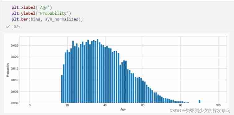
Our strategy is simple ： We count every histogram bar ; We will normalize these counts , Let their sum be 1, Then treat them as probabilities .

Once we have these probabilities , We can go through Randomly select a bar of the histogram , Weighted by probability , Sample from the distribution it represents . Our first step is to prepare for counting , The method is to ensure that no count is negative , And normalize them into 1：

dp_syn_rep_nn = np.clip(dp_syn_rep, 0, None)
syn_normalized = dp_syn_rep_nn / np.sum(dp_syn_rep_nn)
np.sum(syn_normalized)

Please note that , If we plot normalized counts - We can now think of it as the probability of each corresponding histogram bar , Because the sum of them is 1 - We see a shape that looks very much like the original histogram （ In turn, , It looks like the shape of the original data ）. This is all predictable - In addition to their size , These probabilities are just counts .

plt.xlabel('Age')
plt.ylabel('Probability')
plt.bar(bins, syn_normalized);

The last step is to generate new samples based on these probabilities . We can use np.random.choice, It allows you to pass in a list of probabilities associated with the selection given in the first parameter （ In the parameters ）. It accurately realizes the weighted random selection required by the sampling task . We can generate any number of samples as needed , Without additional privacy costs , Because we have set the count to differential privacy .

def gen_samples(n):
    return np.random.choice(bins, n, p=syn_normalized)

syn_data = pd.DataFrame(gen_samples(5), columns=['Age'])
syn_data

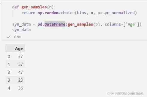
We hope , The samples we generate in this way will be roughly distributed according to the same basic distribution as the original data . This means that we can use the generated comprehensive data to answer the same query that can be answered with the original data . especially , If we plot the age histogram in a large synthetic data set , We will see the same shape as the original data .

syn_data = pd.DataFrame(gen_samples(10000), columns=['Age'])
plt.xlabel('Age')
plt.ylabel('Number of Occurrences')
plt.hist(syn_data['Age'], bins=bins);

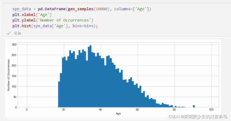
We can also answer other queries we have seen in the past , For example, average value and range query ：

print('Mean age, synthetic: {}'.format(np.mean(syn_data['Age'])))
print('Mean age, true answer: {}'.format(np.mean(adult['Age'])))
print('Percent error: {}'.format(pct_error(np.mean(syn_data['Age']), np.mean(adult['Age']))))

print('Mean age, synthetic: {}'.format(range_query(syn_data, 'Age', 20, 65)))
print('Mean age, true answer: {}'.format(range_query(adult, 'Age', 20, 65)))
print('Percent error: {}'.format(pct_error(range_query(adult, 'Age', 20, 65), 
                                           range_query(syn_data, 'Age', 20, 65))))

Our mean query has a fairly low error （ Although the error is still much larger than what we can achieve by directly applying the Laplace mechanism ）.

however , Our range query has a very big error ！ This is only because we don't exactly match the shape of the original data - We only generated 10,000 Samples , The original data set has more than 30,000 That's ok . We can perform additional differential private queries to determine the number of rows in the original data , Then generate a new comprehensive data set with the same number of rows , This will improve our range query results .

n = laplace_mech(len(adult), 1, 1.0)
syn_data = pd.DataFrame(gen_samples(int(n)), columns=['Age'])

print('Mean age, synthetic: {}'.format(range_query(syn_data, 'Age', 20, 65)))
print('Mean age, true answer: {}'.format(range_query(adult, 'Age', 20, 65)))
print('Percent error: {}'.format(pct_error(range_query(adult, 'Age', 20, 65), 
                                           range_query(syn_data, 'Age', 20, 65))))

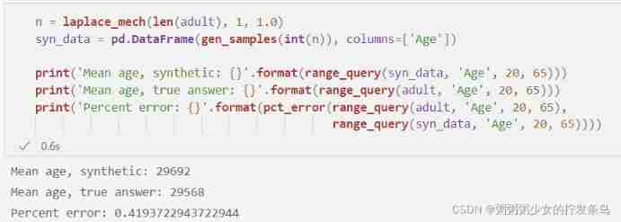
Now we see the lower error we expect .

Generate more columns

up to now , We have generated comprehensive data that matches the number of rows in the original data set , And it is very useful for answering queries about raw data , But it has only one column ！ How can we generate more columns ？

There are two basic ways .

We can deal with every $k$ Column repeats the process followed above （ Generate $k$ 1 To the margin 【1-way marginals】）, And come to $k$ Separate synthetic datasets , Each data set has a column . then , We can decompose these data sets , To construct with $k$ A single dataset of columns . This method is very simple , But since we consider each column in isolation , Therefore, we will lose the correlation between the columns in the original data . for example , In the data , Age and occupation may be related （ for example , Managers are more likely to be older than younger ）; If we consider each column in isolation , We will get the right 18 Age and number of managers , But we may be right 18 The number of year-old managers is very wrong .

Another way is to put multiple columns together . for example , We can consider both age and occupation , And calculate how many 18 Year old manager , How many? 19 Year old manager , wait . The result of this modification process is a two-way marginal distribution . We will eventually consider all possible combinations of age and occupation - This is exactly what we did when building the emergency table ！ for example ：

ct = pd.crosstab(adult['Age'], adult['Occupation'])
ct.head()

Now? , We can completely follow the previous practice - Add noise to these counts , Then normalize them and treat them as probabilities ！ Now? , Each count corresponds to a pair of values - Age and occupation - therefore , When we sample from the constructed distribution , We will get two values at the same time .

dp_ct = ct.applymap(lambda x: max(laplace_mech(x, 1, 1), 0))
dp_vals = dp_ct.stack().reset_index().values.tolist()
probs = [p for _,_,p in dp_vals]
vals = [(a,b) for a,b,_ in dp_vals]
probs_norm = probs / np.sum(probs)
list(zip(vals, probs_norm))[0]

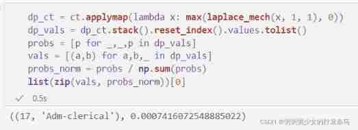
Check the first element of probability , We found that we have 0.07% Opportunity generation represents 17 Years old clerical workers . Now? , We are ready to generate some rows ！ We're going to start with vals Generate an index list from the list , Then index to vals; We have to do this , because np.random.choice The tuple list in the first parameter is not accepted .

indices = range(0, len(vals))
n = laplace_mech(len(adult), 1, 1.0)
gen_indices = np.random.choice(indices, int(n), p=probs_norm)
syn_data = [vals[i] for i in gen_indices]

syn_df = pd.DataFrame(syn_data, columns=['Age', 'Occupation'])
syn_df.head()

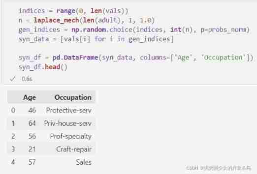
The disadvantage of considering both columns at the same time is that our accuracy will be lower . When we add more columns to the set under consideration （ namely , Construct a $n$ To the margin , increase $n$ Value ）, We see the same effect as for contingency tables - Each count gets smaller , Therefore, the signal becomes smaller relative to the noise , And our results are not so accurate . We can see this effect by plotting the age histogram in the new synthetic data set ; Please note that , It has roughly the right shape , But it is not as smooth as the raw data or the difference private count we use for the age series itself .

plt.xlabel('Age')
plt.ylabel('Number of Occurrences')
plt.hist(syn_df['Age'], bins=bins);

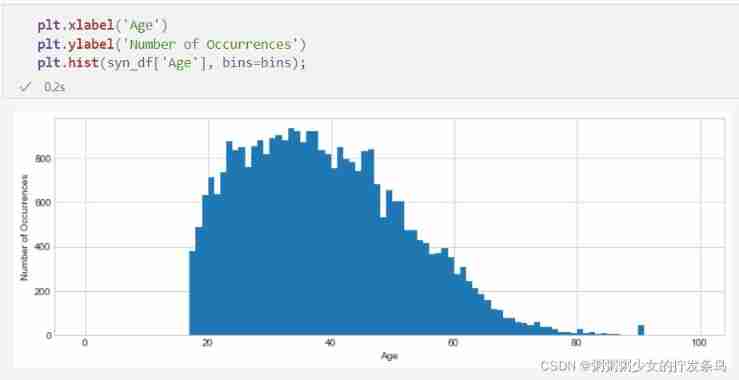
When we try a specific query only for the age column , We will see the same loss of accuracy ：

real_answer = range_query(adult, 'Age', 20, 30)
syn_answer = range_query(syn_df, 'Age', 20, 30)
print('Percent error using synthetic data:', pct_error(real_answer, syn_answer))

summary

1、 A comprehensive representation of the dataset allows you to answer queries about the original data

2、 A common example of a composite representation is a histogram , It can be made differential privacy by adding noise to its count

3、 Histogram representation can be used to generate synthetic data with the same shape as the original data , The method is to regard its count as probability ： Normalize the count to 1, Then, the corresponding normalized count is used as the probability to sample from the histogram bar

4、 Normalized histogram is the representation of one-way marginal distribution , It captures information in a single column in isolation

5、 One way margin does not capture the correlation between columns

6、 To generate multiple columns , We can use multiple one-way margins , Or we can construct a $n$ The representation of bit margin , among $n>1$

7、 With $n$ The growth of , Differential equation $n$ The road edge becomes more and more noisy , Because the bigger $n$ It means that the count of each column of the generated histogram is smaller

8、 therefore , The challenging trade-off for generating synthetic data is ： Using multiple one-way edges will lose the correlation between columns \ Using a single $n$ The way margin is often very inaccurate

9、 in many instances , It may not be possible to generate synthetic data that is both accurate and captures important correlations between columns .