当前位置:网站首页>MATLB | real time opportunity constrained decision making and its application in power system
MATLB | real time opportunity constrained decision making and its application in power system
2022-07-06 01:16:00 【Power system code】
Catalog
2.1 Situational approach to opportunity constrained decision making
2.2 Scenario method with measurement
3、 ... and 、 A fast method of opportunity constrained decision making
3.1 Approximate adjustment through affine transformation
3.2 Affine transformation of feasible region
3.3 Two stage decision algorithm
Four 、 Numerical example —— Power distribution network
4.1 Prevent the active power reduction of overvoltage

Column directory query :* The beauty of power system and algorithm (Python&Matlab Code )
One 、 summary
Many engineering problems can be expressed as decision-making examples under uncertainty , That is, when the problem parameters are uncertain , The problem of making cost-effective decisions that satisfy certain given constraints . A natural approach is to make a decision that ensures that any possible acceptable value for an unknown parameter is feasible , So take the worst-case paradigm . In some applications , This robust approach produces programs that are easy to handle , You can find the best solution . Such a solution may be very conservative in terms of achievable performance : The decision may be affected by the extreme value of the parameter , These extreme values are extremely unlikely, but they have a serious impact on the feasible region for seeking the optimal decision .
The second method is to formulate the so-called opportunity constrained decision-making problem . In these questions , It can be tolerated that a set of parameter values with the minimum probability measure in the parameter space can violate the constraints of the problem , Therefore, it is unlikely to achieve . This approach allows for security ( Aimed at the probability of violating the constraint ) And performance ( Cost of decision ) Weigh against . Chance constrained problems are usually nonconvex and difficult to solve , Even if the original problem with known parameter values is convex . However , They can be effectively solved by adopting the so-called scenario method , Random constraints are replaced by deterministic constraints , By sampling the parameter uncertainty . If the number of constraints is large enough , Then the feasibility in the sense of opportunity constraint can be guaranteed with high confidence . contrary , It can also guarantee the cost of the solution obtained by this method .
In this paper , We consider the chance constrained decision-making problem with a specific structure : One side , We assume that some prior information about the unknown parameters of the decision problem is known , Exist in the form of samples ; On the other hand , We assume that further information about the true values of these parameters can be collected through measurements . We specialize in the scenario approach , So that prior samples and available metrics can be used effectively , To generate feasible regions that meet opportunity constraints . This leads to a two-stage algorithm , It consists of offline pretreatment of samples , Then there is the online part , It needs to be carried out immediately when the measurement is available . The online part is very lightweight in terms of computing time and memory consumption , Therefore, it is suitable for implementation in embedded systems . As an application of choice , We consider the control of micro generators in Distribution Networks .
In the second section , We briefly reviewed the scenario approach , The decision-making problem with limited opportunities is formulated by measurement . In the third section , Shows how to approximate the posterior distribution of unknown parameters , And a fast algorithm for solving chance constrained decision-making problem is analyzed . In section four , It shows the effectiveness of the proposed real-time operation algorithm of distribution network .
Two 、 mathematical model
2.1 Situational approach to opportunity constrained decision making
Consider opportunity constrained decision making :

among x ∈ Rn It's a decision variable ,f (x) It's convex cost , Are unknown disturbances modeled as random variables ,
 It's a constant term . Let's assume that random variables w The support of is given a σ - Algebra. D also P stay D Defined on the . Last , ∈ (0, 1) Is the expected probability of violating the constraint .
The general chance constrained decision problem is nonconvex , And it is usually difficult to deal with in calculation . Please note that , We assume that linear constraints are affine in random variables . under these circumstances , as long as w The basic distribution of is known , You can get the analysis results , Provide conditions for the opportunity constrained problem to be reformulated as a convex problem . In any other case , Scenario methods are all about transforming random programs into deterministic problems in this form :

among  It is a random disturbance N Samples . If N Large enough , Then this mathematical description is equivalent to the above one .
The scene method is obviously not distributed , This means that there is no interference w Make any assumptions about the probability distribution . By the amount that needs to be sampled according to such a distribution  , About w The distributed information still exists implicitly . This feature of the scene method makes it impossible to obtain a reliable interference first principle model , But applications that can use historical data are very attractive .
2.2 Scenario method with measurement
In some applications , About interference w Online information may be available . for example , Although it may be possible to obtain information about w Prior information of distribution , But some direct measurements may be made when making a decision . We formalize the opportunity constrained decision-making problem with measurement as :
among y = Hw It is a linear measurement of disturbance , among H It is the rank of the whole bank ,![\mathbb{P}[\cdot \mid \cdot]](http://img.inotgo.com/imagesLocal/202207/06/202207060112178722_3.gif) The conditional probability . Direct application of scenario method , Such as (3) Medium , The deterministic optimization equation in the following form will be generated :
The conditional probability . Direct application of scenario method , Such as (3) Medium , The deterministic optimization equation in the following form will be generated :

among  Is measured by y = Hw Samples of the determined conditional probability distribution .
The last setting seems to offset the effectiveness of the real-time operation scenario method , Because samples 
Only in measurement y You need to generate . The use of historical samples makes the integration of this new information difficult . Besides , The resulting optimization problem (5) There are still a lot of typical redundancy constraints , This poses a computational challenge to the direct use of scenario methods for fast real-time decision-making . In the next section , We will show how to successfully solve these two problems through the offline preprocessing phase of the sample , Then there is the decision-making step driven by online measurement .
3、 ... and 、 A fast method of opportunity constrained decision making
3.1 Approximate adjustment through affine transformation
3.2 Affine transformation of feasible region
3.3 Two stage decision algorithm
Four 、 Numerical example —— Power distribution network
4.1 Prevent the active power reduction of overvoltage
4.2 Numerical simulation
4.3 Matlab Realization
Only part of the code is shown here , See : We are shipping your work details
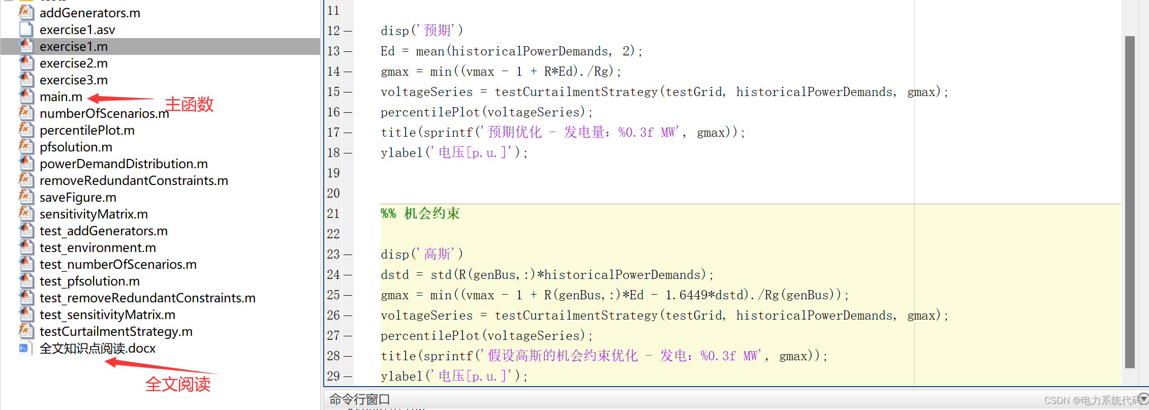
%% ==== Robust optimization ===========

disp(' Robust ')
gmax = (vmax - 1) / max(Rg);
voltageSeries = testCurtailmentStrategy(testGrid, historicalPowerDemands, gmax);
percentilePlot(voltageSeries);
title(sprintf(' Robust optimization —— Power generation :% 0.3f MW', gmax));
ylabel(' voltage  [p.u.]');

%%  expect

disp(' expect ')
Ed = mean(historicalPowerDemands, 2);
gmax = min((vmax - 1 + R*Ed)./Rg);
voltageSeries = testCurtailmentStrategy(testGrid, historicalPowerDemands, gmax);
percentilePlot(voltageSeries);
title(sprintf(' Expected optimization  -  Power generation :%0.3f MW', gmax));
ylabel(' voltage [p.u.]');


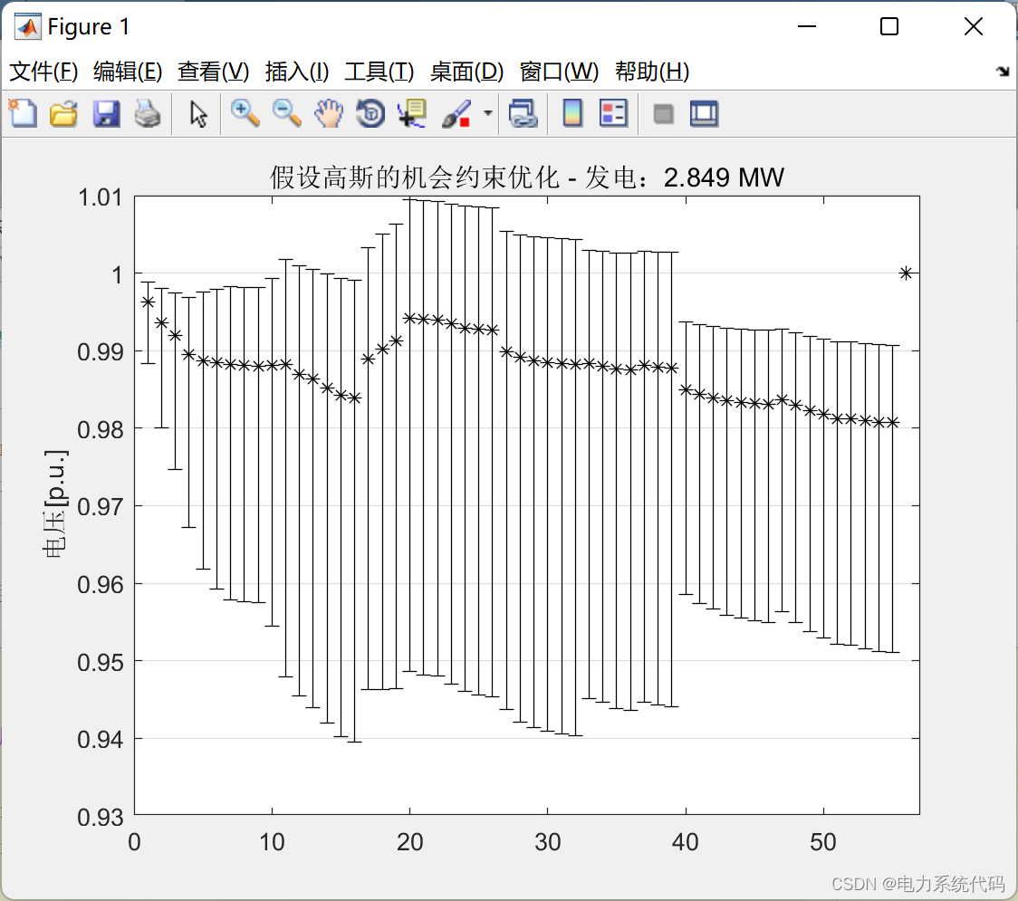
%%  Opportunity constraints

disp(' gaussian ')
dstd = std(R(genBus,:)*historicalPowerDemands);
gmax = min((vmax - 1 + R(genBus,:)*Ed - 1.6449*dstd)./Rg(genBus));
voltageSeries = testCurtailmentStrategy(testGrid, historicalPowerDemands, gmax);
percentilePlot(voltageSeries);
title(sprintf(' Suppose Gauss's chance constrained optimization  -  Electricity generation :%0.3f MW', gmax));
ylabel(' voltage [p.u.]');
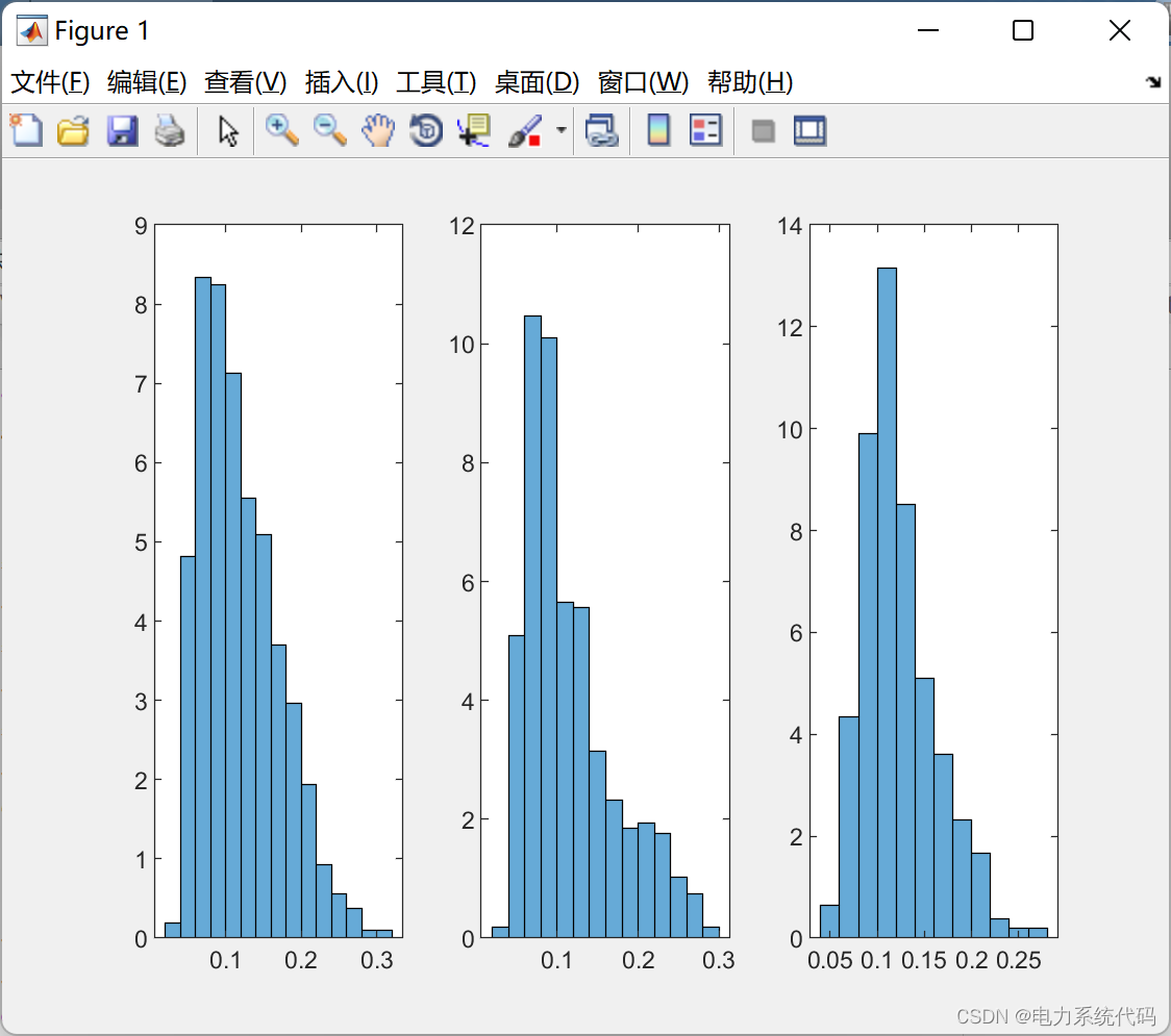
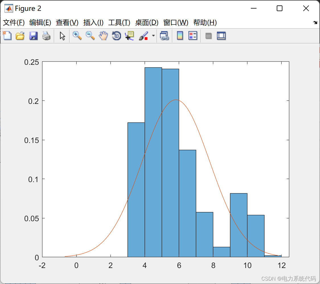
4.4 Running results

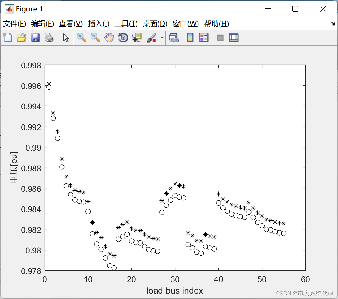
边栏推荐
- 3D模型格式汇总
- 朝招金安全吗 会不会亏损本金
- Cf:c. the third problem
- C language programming (Chapter 6 functions)
- GNSS terminology
- Dynamic programming -- linear DP
- How to extract MP3 audio from MP4 video files?
- General operation method of spot Silver
- Dede collection plug-in free collection release push plug-in
- Study diary: February 13, 2022
猜你喜欢
Dede collection plug-in free collection release push plug-in
cf:H. Maximal AND【位运算练习 + k次操作 + 最大And】

Beginner redis
Convert binary search tree into cumulative tree (reverse middle order traversal)
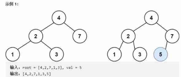
Recursive method to realize the insertion operation in binary search tree

Questions about database: (5) query the barcode, location and reader number of each book in the inventory table
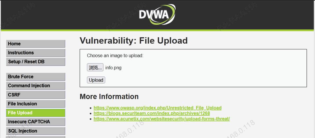
Test de vulnérabilité de téléchargement de fichiers basé sur dvwa

Vulhub vulnerability recurrence 75_ XStream

伦敦银走势中的假突破

MATLB|实时机会约束决策及其在电力系统中的应用
随机推荐
Getting started with devkit
MobileNet系列(5):使用pytorch搭建MobileNetV3并基于迁移学习训练
ubantu 查看cudnn和cuda的版本
Mysql--- query the top 5 students
The inconsistency between the versions of dynamic library and static library will lead to bugs
普通人下场全球贸易,新一轮结构性机会浮出水面
The population logic of the request to read product data on the sap Spartacus home page
Paging of a scratch (page turning processing)
面试必刷算法TOP101之回溯篇 TOP34
Hcip---ipv6 experiment
MIT doctoral thesis | robust and reliable intelligent system using neural symbol learning
Who knows how to modify the data type accuracy of the columns in the database table of Damon
Leetcode 208. 实现 Trie (前缀树)
China Taiwan strategy - Chapter 8: digital marketing assisted by China Taiwan
Cannot resolve symbol error
Netease smart enterprises enter the market against the trend, and there is a new possibility for game industrialization
Building core knowledge points
BiShe - College Student Association Management System Based on SSM
cf:C. The Third Problem【关于排列这件事】
Zhuhai laboratory ventilation system construction and installation instructions