当前位置:网站首页>Nonlinear optimization: steepest descent method, Newton method, Gauss Newton method, Levenberg Marquardt method
Nonlinear optimization: steepest descent method, Newton method, Gauss Newton method, Levenberg Marquardt method
2022-07-02 10:19:00 【Jason. Li_ 0012】
Nonlinear optimization
For a minimum nonlinear multiplication problem :
min x F ( x ) = 1 2 ∥ f ( x ) ∥ 2 2 \min_xF(x)=\frac{1}{2}\begin{Vmatrix}f(x)\end{Vmatrix}^2_2 xminF(x)=21∥∥f(x)∥∥22
Find the function in the formula f ( x ) f(x) f(x) Of L2 The minimum value of half of the sum of squares of norms ,L2 Norm refers to the square operation after taking the sum of squares of each item .
Solve the minimum objective function , Into the independent variable when its derivative is zero x x x Value :
d F d x = 0 \frac{dF}{dx}=0 dxdF=0
It is generally used iteration To solve , Start with an initial value , Update variables iteratively , Make the value of the objective function drop :
1. to set first beginning value x 0 2. Yes On The first k Time Overlapping generation , Look for look for increase The amount Δ x k send have to ∥ f ( x k + Δ x k ) ∥ 2 2 reach To extremely Small value 3. if Δ x k foot enough Small , be full foot strip Pieces of stop stop 4. back And , x k + 1 = x k + Δ x k , Following To continue Overlapping generation Next One round \begin{aligned} 1.& Given the initial value x_0\\ 2.& For the first k Sub iteration , Look for increments \Delta x_k bring \begin{Vmatrix}f(x_k+\Delta x_k)\end{Vmatrix}^2_2 To reach a minimum \\ 3.& if \Delta x_k Small enough , If the condition is met, stop \\ 4.& conversely ,x_{k+1}=x_k+\Delta x_k, Continue iteration for the next round \\ \end{aligned} 1.2.3.4. to set first beginning value x0 Yes On The first k Time Overlapping generation , Look for look for increase The amount Δxk send have to ∥∥f(xk+Δxk)∥∥22 reach To extremely Small value if Δxk foot enough Small , be full foot strip Pieces of stop stop back And ,xk+1=xk+Δxk, Following To continue Overlapping generation Next One round
Solve increment Δ x k \Delta x_k Δxk The way , There are usually the following : The steepest descent 、 Newton method 、 gaussian - Newton's method and lewenberg - Marquardt method et al .
The steepest descent
Consider the k k k Sub iteration , Make the objective function First order Taylor expansion :
F ( x k + Δ x k ) ≈ F ( x k ) + J ( x k ) T Δ x k F(x_k+\Delta x_k)\approx F(x_k)+J(x_k)^T\Delta x_k F(xk+Δxk)≈F(xk)+J(xk)TΔxk
matrix J ( x k ) J(x_k) J(xk) For the function F ( x ) F(x) F(x) About x x x First derivative of , be called Jacobian matrix (Jacobian Matrix).
At this time, you can select the increment as follows :
Δ x ∗ = a r g min ( F ( x k ) + J ( x k ) T Δ x k ) \Delta x^*=arg\min\Bigl(F(x_k)+J(x_k)^T\Delta x_k\Bigr) Δx∗=argmin(F(xk)+J(xk)TΔxk)
Right side to $\Delta x_k $ Derivation and zero :
Δ x ∗ = − J ( x k ) \Delta x^*=-J(x_k) Δx∗=−J(xk)
Usually , A step size needs to be further defined λ \lambda λ, So as to advance along the direction gradient , Make the objective function descend under the first-order linear approximation . The steepest descent method is too greedy , As a result, its descent route is easy to form a sawtooth route ( Go to the edge of the grid ), Thus increasing the number of iterations .
Newton method
Consider the k k k Sub iteration , Make the objective function Second order Taylor expansion :
F ( x k + Δ x k ) ≈ F ( x k ) + J ( x k ) T Δ x k + 1 2 Δ x k T H ( x k ) Δ x k F(x_k+\Delta x_k)\approx F(x_k)+J(x_k)^T\Delta x_k+\frac{1}{2}\Delta x_k^TH(x_k)\Delta x_k F(xk+Δxk)≈F(xk)+J(xk)TΔxk+21ΔxkTH(xk)Δxk
matrix H ( x k ) H(x_k) H(xk) For the function F ( x ) F(x) F(x) About x x x The second derivative of , be called Hazen matrix (Hessian Matrix), At this time, the increment is as follows :
Δ x ∗ = a r g min ( F ( x k ) + J ( x k ) T Δ x k + 1 2 Δ x k T H ( x k ) Δ x k ) \Delta x^*=arg\min\Bigl( F(x_k)+J(x_k)^T\Delta x_k+\frac{1}{2}\Delta x_k^TH(x_k)\Delta x_k\Bigr) Δx∗=argmin(F(xk)+J(xk)TΔxk+21ΔxkTH(xk)Δxk)
Again , The right derivative takes zero :
H ( x k ) Δ x k = − J ( x k ) H(x_k)\Delta x_k=-J(x_k) H(xk)Δxk=−J(xk)
Solve the above linear equation , You can get the incremental expression . Newton's method requires a lot of computational effort to solve H H H, This problem should be avoided .
The quasi Newton method is usually used to solve the least square problem .
gaussian - Newton method
For an objective function F ( x ) F(x) F(x):
min x F ( x ) = 1 2 ∥ f ( x ) ∥ 2 2 \min_xF(x)=\frac{1}{2}\begin{Vmatrix}f(x)\end{Vmatrix}^2_2 xminF(x)=21∥∥f(x)∥∥22
Gauss Newton method passes f ( x ) f(x) f(x) Do Taylor expansion , Instead of F ( x ) F(x) F(x) Target expansion , To improve efficiency .
f ( x k + Δ x k ) ≈ f ( x k ) + J ( x k ) T Δ x k f(x_k+\Delta x_k)\approx f(x_k)+J(x_k)^T\Delta x_k f(xk+Δxk)≈f(xk)+J(xk)TΔxk
here , Solve the increment so that ∥ f ( x + Δ x k ) ∥ 2 \begin{Vmatrix}f(x+\Delta x_k)\end{Vmatrix}^2 ∥∥f(x+Δxk)∥∥2 Minimum :
Δ x ∗ = a r g min x 1 2 ∥ f ( x k ) + J ( x k ) T Δ x k ∥ 2 \Delta x^* = arg\min_{x}\frac{1}{2}\begin{Vmatrix}f(x_k)+J(x_k)^T\Delta x_k\end{Vmatrix}^2 Δx∗=argxmin21∥∥f(xk)+J(xk)TΔxk∥∥2
Simplify the expression :
1 2 ∥ f ( x k ) + J ( x k ) T Δ x k ∥ 2 = 1 2 ( f ( x k ) + J ( x k ) T Δ x k ) T ( f ( x k ) + J ( x k ) T Δ x k ) = 1 2 ( ∥ f ( x k ) ∥ 2 2 + 2 f ( x k ) J ( x ) T Δ x k + Δ x k T J ( x k ) J ( x k ) T Δ x k ) \begin{aligned} \frac{1}{2}\begin{Vmatrix}f(x_k)+J(x_k)^T\Delta x_k\end{Vmatrix}^2&=\frac{1}{2}\Bigl(f(x_k)+J(x_k)^T\Delta x_k\Bigr)^T\Bigl(f(x_k)+J(x_k)^T\Delta x_k\Bigr)\\ &=\frac{1}{2}\Bigl(\begin{Vmatrix}f(x_k)\end{Vmatrix}^2_2+2f(x_k)J(x)^T\Delta x_k+\Delta x_k^TJ(x_k)J(x_k)^T\Delta x_k\Bigr) \end{aligned} 21∥∥f(xk)+J(xk)TΔxk∥∥2=21(f(xk)+J(xk)TΔxk)T(f(xk)+J(xk)TΔxk)=21(∥∥f(xk)∥∥22+2f(xk)J(x)TΔxk+ΔxkTJ(xk)J(xk)TΔxk)
Solve to minimize x x x That's right Δ x \Delta x Δx The derivative is zero :
J ( x k ) f ( x k ) + J ( x k ) J T ( x k ) Δ x k = 0 J ( x k ) J T ( x k ) Δ x k = − J ( x k ) f ( x k ) \begin{aligned} J(x_k)f(x_k)+J(x_k)J^T(x_k)\Delta x_k =0\\ J(x_k)J^T(x_k)\Delta x_k=-J(x_k)f(x_k) \end{aligned} J(xk)f(xk)+J(xk)JT(xk)Δxk=0J(xk)JT(xk)Δxk=−J(xk)f(xk)
remember H ( x k ) = J ( x k ) J T ( x k ) H(x_k)=J(x_k)J^T(x_k) H(xk)=J(xk)JT(xk), g ( x k ) = − J ( x k ) f ( x k ) g(x_k)=-J(x_k)f(x_k) g(xk)=−J(xk)f(xk), So as to get information about Δ x k \Delta x_k Δxk A linear system of equations :
H ( x k ) Δ x k = g ( x k ) H(x_k)\Delta x_k=g(x_k) H(xk)Δxk=g(xk)
Call it The incremental equation , or Gauss Newton equation (Gauss-Newton Equation), Normal equation (Normal Equation). gaussian - Newton's method uses J J T JJ^T JJT Second order Hessian matrix in approximate Newton method H H H, So as to avoid a lot of calculations , The algorithm flow is as follows :
1. to set first beginning value x 0 2. Yes The first k Time Overlapping generation , seek Jas. can Than Moment front J ( x k ) and By mistake Bad f ( x k ) 3. seek Explain increase The amount Fang cheng : H Δ x k = g 4. if Δ x k foot enough Small , be full foot strip Pieces of stop stop 5. back And , x k + 1 = x k + Δ x k , Following To continue Overlapping generation Next One round \begin{aligned} 1.& Given the initial value x_0\\ 2.& Right. k Sub iteration , Find the Jacobian matrix J(x_k) And error f(x_k)\\ 3.& Solving the incremental equation :H\Delta x_k=g\\ 4.& if \Delta x_k Small enough , If the condition is met, stop \\ 5.& conversely ,x_{k+1}=x_k+\Delta x_k, Continue iteration for the next round \\ \end{aligned} 1.2.3.4.5. to set first beginning value x0 Yes The first k Time Overlapping generation , seek Jas. can Than Moment front J(xk) and By mistake Bad f(xk) seek Explain increase The amount Fang cheng :HΔxk=g if Δxk foot enough Small , be full foot strip Pieces of stop stop back And ,xk+1=xk+Δxk, Following To continue Overlapping generation Next One round
For the solution of incremental equation , The matrix should be satisfied H H H reversible , but J J T JJ^T JJT Is a positive semidefinite matrix , Singular matrices or ill conditioned situations may occur , This leads to the non convergence of the algorithm . Levenberg - Marquardt method corrects the above problem to a certain extent .
Levenberg - The Marquardt method
Levenberg - The convergence speed of Marquardt method is slower than Gauss - Newton method , But it is more robust , Also known as damped newton method (Damped Newton Method)
gaussian - Newton's second-order Taylor expansion to approximate linearization , Its effect only has a good approximate effect near the expansion point . So deal with Δ x k \Delta x_k Δxk Add an interval range , be called Confidence interval (Trust Region). It is considered that it is approximately valid within the confidence interval and invalid outside the approximate interval .
The difference between the approximate model and the actual function is used to determine the scope of the confidence interval :
ρ = f ( x k + Δ x k ) − f ( x k ) J ( x k ) T Δ x \rho=\frac{f(x_k+\Delta x_k)-f(x_k)}{J(x_k)^T\Delta x} ρ=J(xk)TΔxf(xk+Δxk)−f(xk)
indicators ρ \rho ρ Used to describe the good or bad degree of approximation , among , The denominator is the value decreased by the approximate model , The numerator is the decreasing value of the actual function .
ρ \rho ρ near 1, The approximate effect is good , The approximate range should be expanded ; ρ \rho ρ smaller , The approximation effect is poor , The approximate range should be reduced . thus , Build Levenberg - Marquardt algorithm model :
1. to set first beginning value x 0 With And first beginning optimal turn And a half path μ 2. Yes The first k Time Overlapping generation , stay high Si cattle Ton Law Of The base Foundation On increase Add Letter lai District Domain : min Δ x k 1 2 ∥ f ( x k ) + J ( x k ) T Δ x k ∥ 2 , s . t . ∥ D Δ x k ∥ 2 ≤ μ , Its in , μ by Letter lai District between And a half path , D by system Count Moment front 3. meter count finger mark : ρ = f ( x k + Δ x k ) − f ( x k ) J ( x k ) T Δ x 4. if ρ > 0.75 , be set up Set up μ = 2 μ 5. if ρ < 0.25 , be set up Set up μ = 0.5 μ 6. if ρ It's about On some threshold value District between , be recognize by near like can That's ok , x k + 1 = x k + Δ x k 7. sentence break yes no closed Convergence , if closed Convergence be junction beam , back And return return The first Two Step Overlapping generation \begin{aligned} 1.& Given the initial value x_0 And the initial optimization radius \mu\\ 2.& Right. k Sub iteration , The trust region is added on the basis of Gauss Newton method :\\ &\qquad\qquad\min_{\Delta x_k}\frac{1}{2}\begin{Vmatrix}f(x_k)+J(x_k)^T\Delta x_k\end{Vmatrix}^2,\quad s.t.\quad \begin{Vmatrix}D\Delta x_k\end{Vmatrix}^2\leq\mu, \\ &\qquad\qquad among ,\mu Is the radius of the confidence interval ,D Is the coefficient matrix \\ 3.& Calculate the index :\rho=\frac{f(x_k+\Delta x_k)-f(x_k)}{J(x_k)^T\Delta x}\\ 4.& if \rho>0.75, Is set \mu=2\mu\\ 5.& if \rho<0.25, Is set \mu=0.5\mu\\ 6.& if \rho In a certain threshold range , It is considered to be approximately feasible ,x_{k+1}=x_k+\Delta x_k\\ 7.& Judge whether convergence or not , If it converges, it ends , Otherwise, return to the second iteration \\ \end{aligned} 1.2.3.4.5.6.7. to set first beginning value x0 With And first beginning optimal turn And a half path μ Yes The first k Time Overlapping generation , stay high Si cattle Ton Law Of The base Foundation On increase Add Letter lai District Domain :Δxkmin21∥∥f(xk)+J(xk)TΔxk∥∥2,s.t.∥∥DΔxk∥∥2≤μ, Its in ,μ by Letter lai District between And a half path ,D by system Count Moment front meter count finger mark :ρ=J(xk)TΔxf(xk+Δxk)−f(xk) if ρ>0.75, be set up Set up μ=2μ if ρ<0.25, be set up Set up μ=0.5μ if ρ It's about On some threshold value District between , be recognize by near like can That's ok ,xk+1=xk+Δxk sentence break yes no closed Convergence , if closed Convergence be junction beam , back And return return The first Two Step Overlapping generation
here , Limit the increment value to the radius μ \mu μ In the ball ( ∥ Δ x k ∥ 2 ≤ μ \begin{Vmatrix}\Delta x_k\end{Vmatrix}^2\leq\mu ∥∥Δxk∥∥2≤μ), After adding the coefficient matrix , It can be regarded as an ellipsoid ( ∥ D Δ x k ∥ 2 ≤ μ \begin{Vmatrix}D\Delta x_k\end{Vmatrix}^2\leq\mu ∥∥DΔxk∥∥2≤μ).
Levenberg takes D = I D=I D=I, That is, incremental constraint in the ball . And Marquardt will D D D Take it as a non negative diagonal matrix ( In practice, we usually take J T J J^TJ JTJ Square root of diagonal element ), Thus, the constraint range on the dimension with small gradient is larger .
Construct Lagrange equation , Put the constraint into the objective function :
L ( Δ x k , λ ) = 1 2 ∥ f ( x k ) + J ( x k ) T Δ x k ∥ 2 + λ 2 ( ∥ D Δ x k ∥ 2 − μ ) L(\Delta x_k, \lambda)=\frac{1}{2}\begin{Vmatrix}f(x_k)+J(x_k)^T\Delta x_k\end{Vmatrix}^2+\frac{\lambda}{2}\Bigl(\begin{Vmatrix}D\Delta x_k\end{Vmatrix}^2-\mu\Bigr) L(Δxk,λ)=21∥∥f(xk)+J(xk)TΔxk∥∥2+2λ(∥∥DΔxk∥∥2−μ)
call λ \lambda λ Is the Lagrange multiplier , Ask about Δ x k \Delta x_k Δxk The derivative of is zero :
( H + λ D T D ) Δ x k = g (H+\lambda D^TD)\Delta x_k =g (H+λDTD)Δxk=g
When parameters λ \lambda λ More hours , H H H Occupy a dominant position , The quadratic approximation model is better in the range , Levenberg - Marquardt method is close to Gauss Newton method ; When parameters λ \lambda λ large , λ D T D \lambda D^TD λDTD Occupy a dominant position , The quadratic approximation model is poor in the range , Levenberg - The Marquardt method is close to the steepest descent method . Levenberg - Marquardt method to a certain extent , The coefficient matrix of linear equations can be avoided to be nonsingular 、 Sick questions , Provide more stability 、 More accurate increments Δ x k \Delta x_k Δxk
边栏推荐
- [illusory] automatic door blueprint notes
- MySQL -- time zone / connector / driver type
- 2837xd 代码生成——StateFlow(2)
- Alibaba cloud SMS service
- 渗透测试的介绍和防范
- Data insertion in C language
- 2837xd code generation module learning (4) -- idle_ task、Simulink Coder
- 虚幻——动画蓝图、状态机制作人物走跑跳动作
- 2837xd code generation - stateflow (2)
- Skywalking理论与实践
猜你喜欢
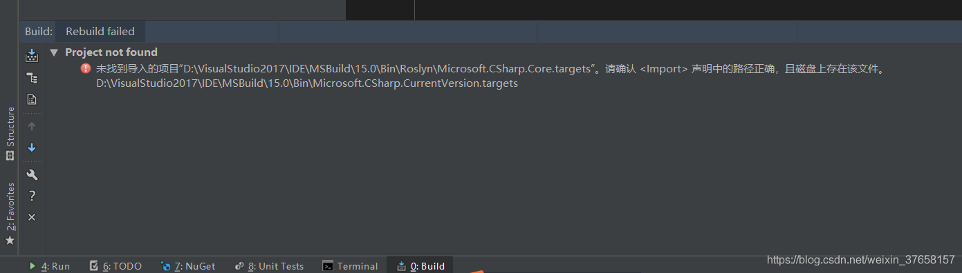
【JetBrain Rider】构建项目出现异常:未找到导入的项目“D:\VisualStudio2017\IDE\MSBuild\15.0\Bin\Roslyn\Microsoft.CSh

Blender volume fog

Unreal material editor foundation - how to connect a basic material

Blender海洋制作
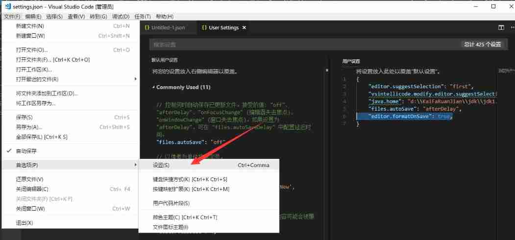
Vscode set JSON file to format automatically after saving

How to judge the quality of primary market projects when the market is depressed?

【UE5】AI随机漫游蓝图两种实现方法(角色蓝图、行为树)
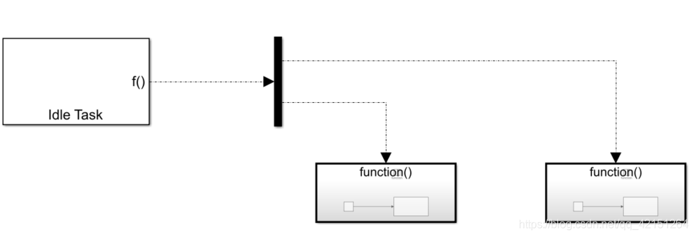
2837xd code generation module learning (4) -- idle_ task、Simulink Coder

Blender多镜头(多机位)切换

2837xd code generation - Supplement (2)
随机推荐
Project practice, redis cluster technology learning (10)
Binary and decimal system of C language
Vscode set JSON file to format automatically after saving
Notes de base sur les plans illusoires d'IA (triés en 10 000 mots)
Project practice, redis cluster technology learning (12)
SAP Spartacus express checkout design
【Unity3D】嵌套使用Layout Group制作拥有动态子物体高度的Scroll View
Junit4 runs MVN test test suite upgrade scheme
Blender stone carving
【UE5】AI随机漫游蓝图两种实现方法(角色蓝图、行为树)
虚幻——动画蓝图、状态机制作人物走跑跳动作
虚幻材质编辑器基础——如何连接一个最基本的材质
高考那些事
Blender volume fog
【虚幻】自动门蓝图笔记
ue虛幻引擎程序化植物生成器設置——如何快速生成大片森林
虚幻AI蓝图基础笔记(万字整理)
【Lua】常见知识点汇总(包含常见面试考点)
职业规划和发展
This monitoring system makes workers tremble: turnover intention and fishing can be monitored. After the dispute, the product page has 404