当前位置:网站首页>从零实现深度学习框架——LSTM从理论到实战【实战】
从零实现深度学习框架——LSTM从理论到实战【实战】
2022-07-05 18:58:00 【愤怒的可乐】
引言
本着“凡我不能创造的,我就不能理解”的思想,本系列文章会基于纯Python以及NumPy从零创建自己的深度学习框架,该框架类似PyTorch能实现自动求导。
要深入理解深度学习,从零开始创建的经验非常重要,从自己可以理解的角度出发,尽量不使用外部完备的框架前提下,实现我们想要的模型。本系列文章的宗旨就是通过这样的过程,让大家切实掌握深度学习底层实现,而不是仅做一个调包侠。
上篇文章中,我们学习了LSTM的理论部分。并且在RNN的实战部分,我们看到了如何实现多层RNN和双向RNN。同样,这里实现的LSTM也支持多层和双向。
LSTMCell
class LSTMCell(Module):
    def __init__(self, input_size, hidden_size: int, bias: bool = True) -> None:
        super(LSTMCell, self).__init__()
        # 组合了 x->input gate; x-> forget gate; x-> g ; x-> output gate 的线性转换
        self.input_trans = Linear(hidden_size, 4 * hidden_size, bias=bias)
        # 组合了 h->input gate; h-> forget gate; h-> g ; h-> output gate 的线性转换
        self.hidden_trans = Linear(input_size, 4 * hidden_size, bias=bias)

    def forward(self, x: Tensor, h: Tensor, c: Tensor) -> Tuple[Tensor, Tensor]:
        # i: input gate
        # f: forget gate
        # o: output gate
        # g: g_t
        ifgo = self.input_trans(h) + self.hidden_trans(x)
        ifgo = F.chunk(ifgo, 4, -1)
        # 一次性计算三个门 与 g_t
        i, f, g, o = ifgo

        c_next = F.sigmoid(f) * c + F.sigmoid(i) * F.tanh(g)

        h_next = F.sigmoid(o) * F.tanh(c_next)

        return h_next, c_next
在实现上参考了最后面的参考文章,将x和h相关的线性变换分开:
i t = Linear x i ( x t ) + Linear h i ( h t − 1 ) f t = Linear x f ( x t ) + Linear h f ( h t − 1 ) g t = Linear x g ( x t ) + Linear h g ( h t − 1 ) o t = Linear x o ( x t ) + Linear h o ( h t − 1 ) (1) \begin{aligned} i_t &= \text{Linear}^i_x(x_t) + \text{Linear}^i_h(h_{t-1}) \\ f_t &= \text{Linear}^f_x(x_t) + \text{Linear}^f_h(h_{t-1}) \\ g_t &= \text{Linear}^g_x(x_t) + \text{Linear}^g_h(h_{t-1}) \\ o_t &= \text{Linear}^o_x(x_t) + \text{Linear}^o_h(h_{t-1}) \\ \end{aligned} \tag{1} itftgtot=Linearxi(xt)+Linearhi(ht−1)=Linearxf(xt)+Linearhf(ht−1)=Linearxg(xt)+Linearhg(ht−1)=Linearxo(xt)+Linearho(ht−1)(1)
比如公式 ( 3 ) (3) (3)的 i t = σ ( U i h t − 1 + W i x t ) i_t = \sigma(U_ih_{t-1} + W_ix_t) it=σ(Uiht−1+Wixt)中 σ \sigma σ的参数部分可以变为:
U i h t − 1 + W i x t ⇒ i t = Linear x i ( x t ) + Linear h i ( h t − 1 ) U_ih_{t-1} + W_ix_t \Rightarrow i_t = \text{Linear}^i_x(x_t) + \text{Linear}^i_h(h_{t-1}) Uiht−1+Wixt⇒it=Linearxi(xt)+Linearhi(ht−1)
然后我们可以组合类似的线性变换,比如组合 x t x_t xt相关的线性变换: Linear x i ( x t ) , Linear x f ( x t ) , Linear x g ( x t ) , Linear x o ( x t ) \text{Linear}^i_x(x_t),\text{Linear}^f_x(x_t),\text{Linear}^g_x(x_t),\text{Linear}^o_x(x_t) Linearxi(xt),Linearxf(xt),Linearxg(xt),Linearxo(xt)为:
self.input_trans = Linear(hidden_size, 4 * hidden_size, bias=bias)
类似地,hidden_trans同理。这样做的原因是为了加快运算速度,我们只需要做一次线性运算,就可以得到四个结果。
通过
ifgo = self.input_trans(h) + self.hidden_trans(x) \tag 2
得到了这四个重要值的结果,但它们拼接到了一个张量中。然后利用
ifgo = F.chunk(ifgo, 4, -1)
将它们拆分成包含四个值的元组,
i, f, g, o = ifgo
这样我们就得到了相应函数里面的参数值,加上对应的Sigmoid函数或Tanh函数就可以得到我们想要的值。
下一步先计算 c t c_t ct:
c t = σ ( f t ) ⊙ c t − 1 + σ ( i t ) ⊙ tanh ( g t ) (3) c_t = \sigma(f_t) \odot c_{t-1} + \sigma(i_t) \odot \tanh(g_t) \tag 3 ct=σ(ft)⊙ct−1+σ(it)⊙tanh(gt)(3)
对应代码:
c_next = F.sigmoid(f) * c + F.sigmoid(i) * F.tanh(g)
然后根据 o t o_t ot和 c t c_t ct计算隐藏状态 h t h_t ht:
h t = σ ( o t ) ⊙ tanh ( c t ) (4) h_t = \sigma(o_t) \odot \tanh(c_t) \tag 4 ht=σ(ot)⊙tanh(ct)(4)
对应代码:
h_next = F.sigmoid(o) * F.tanh(c_next)
LSTM
有了LSTMCell就可以实现完整的LSTM了。
class LSTM(Module):
    def __init__(self, input_size: int, hidden_size: int, batch_first: bool = False, num_layers: int = 1,
                 bidirectional: bool = False, dropout: float = 0):
        super(LSTM, self).__init__()
        self.num_layers = num_layers
        self.hidden_size = hidden_size
        self.batch_first = batch_first
        self.bidirectional = bidirectional

        # 支持多层
        self.cells = ModuleList([LSTMCell(input_size, hidden_size)] +
                                [LSTMCell(hidden_size, hidden_size) for _ in range(num_layers - 1)])

        if self.bidirectional:
            # 支持双向
            self.back_cells = copy.deepcopy(self.cells)

        self.dropout = dropout
        if dropout:
            # Dropout层
            self.dropout_layer = Dropout(dropout)

    def _one_directional_op(self, input, cells, n_steps, hs, cs, reverse=False):
        ''' Args: input: 输入 [n_steps, batch_size, input_size] cells: 正向或反向RNNCell的ModuleList hs: cs: n_steps: 步长 reverse: true 反向 Returns: '''
        output = []
        for t in range(n_steps):
            inp = input[t]

            for layer in range(self.num_layers):
                hs[layer], cs[layer] = cells[layer](inp, hs[layer], cs[layer])
                inp = hs[layer]
                if self.dropout and layer != self.num_layers - 1:
                    inp = self.dropout_layer(inp)

            # 收集最终层的输出
            output.append(hs[-1])

        output = F.stack(output)  # (n_steps, batch_size, num_directions * hidden_size)

        if reverse:
            output = F.flip(output, 0)  # 将输出时间步维度逆序,使得时间步t=0上,是看了整个序列的结果。

        if self.batch_first:
            output = output.transpose((1, 0, 2))

        h_n = F.stack(hs)
        c_n = F.stack(cs)

        return output, (h_n, c_n)

    def forward(self, input: Tensor, state: Optional[Tuple[Tensor, Tensor]] = None):
        ''' Args: input: 形状 [n_steps, batch_size, input_size] 若batch_first=False ;否则形状 [batch_size, n_steps, input_size] state: 元组(h,c) num_directions = 2 if self.bidirectional else 1 h: [num_directions * num_layers, batch_size, hidden_size] c: [num_directions * num_layers, batch_size, hidden_size] Returns: num_directions = 2 if self.bidirectional else 1 output: (n_steps, batch_size, num_directions * hidden_size)若batch_first=False 或 (batch_size, n_steps, num_directions * hidden_size)若batch_first=True 包含每个时间步最后一层(多层RNN)的输出h_t h_n: (num_directions * num_layers, batch_size, hidden_size) 包含最终隐藏状态 c_n: (num_directions * num_layers, batch_size, hidden_size) 包含最终隐藏状态 '''

        h_0, c_0 = None, None
        if state is not None:
            h_0, c_0 = state

        is_batched = input.ndim == 3
        batch_dim = 0 if self.batch_first else 1
        if not is_batched:
            # 转换为批大小为1的输入
            input = input.unsqueeze(batch_dim)
            if state is not None:
                h_0 = h_0.unsqueeze(1)
                c_0 = c_0.unsqueeze(1)

        if self.batch_first:
            batch_size, n_steps, _ = input.shape
            input = input.transpose((1, 0, 2))  # 将batch放到中间维度
        else:
            n_steps, batch_size, _ = input.shape

        if state is None:
            num_directions = 2 if self.bidirectional else 1
            h_0 = Tensor.zeros((self.num_layers * num_directions, batch_size, self.hidden_size), dtype=input.dtype,
                               device=input.device)
            c_0 = Tensor.zeros((self.num_layers * num_directions, batch_size, self.hidden_size), dtype=input.dtype,
                               device=input.device)

        # 得到每层的状态
        hs, cs = list(F.split(h_0)), list(F.split(c_0))

        if not self.bidirectional:
            # 如果是单向的
            output, (h_n, c_n) = self._one_directional_op(input, self.cells, n_steps, hs, cs)
        else:
            output_f, (h_n_f, c_n_f) = self._one_directional_op(input, self.cells, n_steps, hs[:self.num_layers],
                                                                cs[:self.num_layers])

            output_b, (h_n_b, c_n_b) = self._one_directional_op(F.flip(input, 0), self.back_cells, n_steps,
                                                                hs[self.num_layers:], cs[self.num_layers:],
                                                                reverse=True)

            output = F.cat([output_f, output_b], 2)
            h_n = F.cat([h_n_f, h_n_b], 0)
            c_n = F.cat([c_n_f, c_n_b], 0)

        return output, (h_n, c_n)
在多层和双向的实现上和RNN基本一样,其输入输出有些不同。这是由LSTM的架构决定的。
词性标注实战
基于我们上面实现的LSTM来实现该词性标注分类模型,这里同样也叫LSTM:
class LSTM(nn.Module):
    def __init__(self, vocab_size: int, embedding_dim: int, hidden_dim: int, output_dim: int, n_layers: int,
                 dropout: float, bidirectional: bool = False):
        super(LSTM, self).__init__()
        self.embedding = nn.Embedding(vocab_size, embedding_dim)
        self.rnn = nn.LSTM(embedding_dim, hidden_dim, batch_first=True, num_layers=n_layers, dropout=dropout,
                           bidirectional=bidirectional)

        num_directions = 2 if bidirectional else 1
        self.output = nn.Linear(num_directions * hidden_dim, output_dim)

    def forward(self, input: Tensor, hidden: Tensor = None) -> Tensor:
        embeded = self.embedding(input)
        output, _ = self.rnn(embeded, hidden)  # pos tag任务利用的是包含所有时间步的output
        outputs = self.output(output)
        log_probs = F.log_softmax(outputs, axis=-1)
        return log_probs
过程和RNN中的类似,训练代码如下:
embedding_dim = 128
hidden_dim = 128
batch_size = 32
num_epoch = 10
n_layers = 2
dropout = 0.2

# 加载数据
train_data, test_data, vocab, pos_vocab = load_treebank()
train_dataset = RNNDataset(train_data)
test_dataset = RNNDataset(test_data)
train_data_loader = DataLoader(train_dataset, batch_size=batch_size, collate_fn=train_dataset.collate_fn, shuffle=True)
test_data_loader = DataLoader(test_dataset, batch_size=batch_size, collate_fn=test_dataset.collate_fn, shuffle=False)

num_class = len(pos_vocab)

# 加载模型
device = cuda.get_device("cuda:0" if cuda.is_available() else "cpu")
model = LSTM(len(vocab), embedding_dim, hidden_dim, num_class, n_layers, dropout, bidirectional=True)
model.to(device)

# 训练过程
nll_loss = NLLLoss()
optimizer = SGD(model.parameters(), lr=0.1)

model.train()  # 确保应用了dropout
for epoch in range(num_epoch):
    total_loss = 0
    for batch in tqdm(train_data_loader, desc=f"Training Epoch {
      epoch}"):
        inputs, targets, mask = [x.to(device) for x in batch]
        log_probs = model(inputs)
        loss = nll_loss(log_probs[mask], targets[mask])  # 通过bool选择,mask部分不需要计算
        optimizer.zero_grad()
        loss.backward()
        optimizer.step()
        total_loss += loss.item()
    print(f"Loss: {
      total_loss:.2f}")

# 测试过程
acc = 0
total = 0
model.eval()  # 不需要dropout
for batch in tqdm(test_data_loader, desc=f"Testing"):
    inputs, targets, mask = [x.to(device) for x in batch]
    with no_grad():
        output = model(inputs)
        acc += (output.argmax(axis=-1).data == targets.data)[mask.data].sum().item()
        total += mask.sum().item()

# 输出在测试集上的准确率
print(f"Acc: {
      acc / total:.2f}")
输出:
Loss: 102.51
Acc: 0.70
同样的配置,测试集上的准确率也是70%,难道需要更多的批次了么。
这里为了演示,只训练了10个批次。
参考
边栏推荐
- Icml2022 | partial and asymmetric comparative learning of out of distribution detection in long tail recognition
- 5年经验Android程序员面试27天,2022程序员进阶宝典
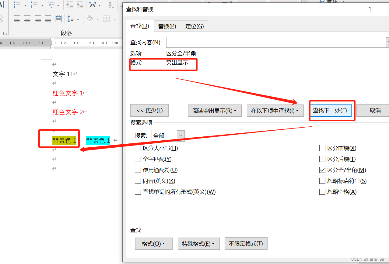
- Word查找红色文字 Word查找颜色字体 Word查找突出格式文本
- 华律网牵手观测云,上线系统全链路可观测平台
- CDB 实例的启动与关闭
- PG基础篇--逻辑结构管理(用户及权限管理)
- The road of enterprise digital transformation starts from here
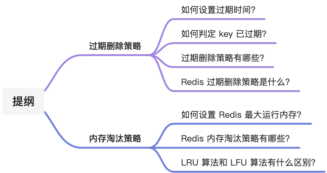
- 面试官:Redis 过期删除策略和内存淘汰策略有什么区别?
- 开源 SPL 消灭数以万计的数据库中间表
- 为什么 BI 软件都搞不定关联分析?带你分析分析
猜你喜欢


随机推荐
Word查找红色文字 Word查找颜色字体 Word查找突出格式文本
跨境支付平台 XTransfer 的低代码实践:如何与其他中台融合是核心
Word finds red text word finds color font word finds highlighted formatted text
Tupu software digital twin smart wind power system
Use file and directory properties and properties
详解SQL中Groupings Sets 语句的功能和底层实现逻辑
Mathematical modeling of oil pipeline layout MATLAB, mathematical model of oil pipeline layout
CF: B. almost Ternary Matrix [symétrie + règles de recherche + Construction + I am Construction Waste]
Video fusion cloud platform easycvr adds multi-level grouping, which can flexibly manage access devices
How to realize the Online timer and offline timer in the game
自动化测试的好处
图扑软件数字孪生 | 基于 BIM 技术的可视化管理系统
Is the performance evaluation of suppliers in the fastener industry cumbersome? Choose the right tool to easily counter attack!
How much does the mlperf list weigh when AI is named?
Debezium系列之:记录mariadb数据库删除多张临时表debezium解析到的消息以及解决方法
Taishan Office Technology Lecture: from the layout height of the line, talk about the height overflow and height shrinkage of the drawing height (launched in the whole network)
Startup and shutdown of CDB instances
The monthly list of Tencent cloud developer community videos was released in May 2022
AI open2022 | overview of recommendation systems based on heterogeneous information networks: concepts, methods, applications and resources
在线协作产品哪家强?微软 Loop 、Notion、FlowUs