当前位置:网站首页>AI zhetianchuan ml novice decision tree
AI zhetianchuan ml novice decision tree
2022-07-08 00:55:00 【Teacher, I forgot my homework】
Decision tree learning is one of the first machine learning methods proposed , Because it is easy to use and has strong interpretability , It is still widely used .
One 、 Decision tree learning foundation
( Relatively simple , Pass by with one )
example : Enjoy a sport

For a new day , Whether you can enjoy sports ?
Classical objective problem for decision tree learning
- Classification problems with non numerical characteristics
- Discrete features
- There is no similarity
- Characteristic disorder
Another example : Fruits
- Color : Red 、 green 、 yellow
- size : Small 、 in 、 Big
- shape : spherical 、 Long and thin
- taste : sweet 、 acid
The sample shows
List of attributes instead of numeric vectors
For example, enjoy sports :
- 6 Value attribute : The weather 、 temperature 、 humidity 、 wind 、 The water temperature 、 Forecast the weather
- A weather example of a day :{ Fine 、 warm 、 commonly 、 strong 、 warm 、 unchanged }
For example, fruit :
- 4 Value tuples : Color 、 size 、 shape 、 taste
- An example of a fruit : { red 、 spherical 、 Small 、 sweet }
The training sample

Decision tree concept
Development history of decision tree - Milepost
• 1966, from Hunt First put forward
• 1970’s~1980’s
• CART from Friedman, Breiman Put forward
• ID3 from Quinlan Put forward
• since 1990’s since
• contrastive study 、 Algorithm improvements (Mingers, Dietterich, Quinlan, etc.)
• The most widely used decision tree algorithm : C4.5 from Quinlan stay 1993 The year of the year
Two 、 Classic decision tree algorithm – ID3
The top-down , Greedy search
A recursive algorithm
Core cycle :
- A : Find the next step The best Decision attributes
- take A As the current node decision attribute
- Pair attribute A (vi ) Each value of , Create a new child node corresponding to it
- The training samples are allocated to each node according to the attribute value
- If The training samples are perfectly classified , Then exit the loop , Otherwise, enter the recursive state and continue to probe down to split the new leaf node
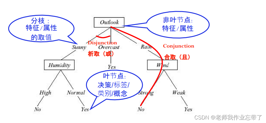
Such as :outlook Is the best decision attribute we found , Let's take it as the current root node , according to outlook That is, we will have different branches and different child nodes according to weather conditions , such as sunny、overcast、rain, If it comes to overcast It's over / There are labels , It means that it has been divided , If it hasn't been divided , We divide a batch of data into sunny、rain On the corresponding branch ,humidity、wind, Enter recursion and continue execution . At this time humidity Is the best attribute we choose .
problem :
- What kind of familiarity is the best decision attribute ?
- What is the perfect classification of training samples ?
Q1: Which attribute is the best ?
For example, there are two properties A1( humidity ) and A2( wind )(64 Data ,29 A good example 35 A negative example )

A1 by true( The humidity is high ) There are 21 just 5 negative by false( Low humidity ) There are 8 just 30 negative
A2 by true( Strong wind ) There are 18 just 33 negative by false( The wind is small ) There are 11 just 2 negative
notes : The positive example is to exercise , The negative example is not going .
At this point in the end A1 and A2( Humidity and wind ) Which is the root node / The best decision attribute is good ?
The basic principle of the current best node selection : concise
---- We prefer to use simple trees with fewer nodes

Pictured above , Suppose there are two kinds of fruits , Watermelon and lemon . We use color color As the root node, it only needs to be based on green still yellow Then we can judge whether it is watermelon or lemon . And if we choose size size , The big one must be watermelon , And the small one may be a small watermelon , So we should judge according to the color .
Attribute selection and node promiscuity (Impurity)
Basic principles of attribute selection : concise
—— We prefer to use simple trees with fewer nodes
At each node N On , We choose an attribute T, Make the data reaching the current derived node as much as possible “ pure ”
The purity (purity) – Promiscuity (impurity)
As shown in the first example above , After Color , Then the green on the left is watermelon, and the yellow on the right is lemon
And in the second Size Small Node , There are watermelon and lemon , It's not enough pure .
How to measure promiscuity ?
1. entropy (Entropy) ( Widely used )


node N The entropy of is expressed as different values under this node  (w: With size Size, for example w1 It's big w2 It's small ,
 by w1 Probability ,
 by w2 Probability .), every last
  The opposite of and .
- Definition : 0log0=0
- In information theory , Entropy measures the purity of information / Promiscuity , Or the uncertainty of information
- It can be seen from the above figure , When entropy is maximum, the probability is half , That is, the most uncertain at this time .
- Normal distribution – Has the largest entropy
Calculate and judge the following example :

You can see A1 A2 All are 29+,35-, Close to half , Entropy should be close to 1 Of .


The blue line :1 The probability of class time is 1,2 The probability of class time is 0.5,16 The probability of class time is 1/16
Red thread :1 The maximum entropy is 0,2 The maximum entropy is 1, Unlimited growth .( The maximum is uniformly distributed )
2. Gini Promiscuity ( Duda Tend to use Gini Promiscuity )
In economics and sociology, people use The gini coefficient To measure the balance of a country's development .

Represents the product of all different cases ( If it is A、B In both cases p(A)*p(B), If it is A、B、C In three cases p(A)*p(B)+p(A)*p(C)+p(B)*p(C))
perhaps 1- The product of the same case ( )
)

n = number of class( It is also because it is evenly distributed , Each part is 1/n)
There is an upper limit , Cap of 1.
3. Misclassification confounding

1- The probability of the largest class , namely 1- Most of the those who enter ( It's right ,1- It's wrong. )

Measure the change of promiscuity -- Information gain (IG)
Due to A The expected reduction of entropy caused by sorting

original S The entropy of - Pass attribute A Expected entropy after classification
 Calculated , so A1( humidity ) Of IG( Information gain ) Bigger , That means we get more information ( The reduced entropy is more ), We choose A1 As root node .
example : Choose which attribute to use as the root node according to the following table 

Outlook Of Gain Maximum , Choose it as the root node .
Q2: When to return ( Stop splitting nodes )?
“ If the training samples are perfectly classified ”
• situation 1: If all data in the current subset There are exactly the same output categories , So stop

• situation 2: If all data in the current subset Have exactly the same input characteristics , So stop
such as : a sunny day - No wind - The humidity is normal - Appropriate temperature , Finally, some went and some didn't . At this point, even if it does not end, there is no way , Because the available information has been used up . It means :1、 The data is noisy noise. Need to be cleaned , If there is too much noise, the data quality is not good enough .2、 Missing important Feature, For example, I missed whether there were classes on that day , There is no way to go out to play when there is a class .
Possible situation 3: If The information gain of all attribute splitting is 0, So stop Is this a good idea ?(No)

As shown in the figure above, the first node of the tree cannot be found at this time (IG All are 0), If 3 That's right , At this time, the decision tree cannot be built .
If we don't want this condition , It's all the same ,IG All are 0, When there are multiple maxima, a random relationship is constructed ( At this time, it is also perfectly classified )

That is to say ID3 Only the above two situations will stop splitting , If IG=0, Just choose one at random .
ID3 The hypothesis space of algorithm search

- Suppose the space is complete ( It can handle both disjunction and conjunction of attributes )
The objective function must be in the hypothesis space
- Output a single hypothesis ( Walk down a path of trees )
No more than 20 A question ( Based on experience , commonly feature No more than 20 individual , If the tree is too complex, it is easy to produce over fitting )
- No backtracking ( With A1 Be the root node , There is no way to return to see A2 How about being a root node )
Local optimum
- Use all the data of the subset in each step ( For example, the weight update strategy in the gradient descent algorithm is to update each data once , That is to use only one piece of data at a time )
Data driven search options
Robust to noise data
ID3 Inductive bias in (Inductive Bias)
- Hypothetical space H It acts on the sample set X Upper
There is no restriction on the hypothetical space
- Prefer trees with greater information gain for attributes close to the root node
Try to find the shortest tree
The bias of the algorithm lies in some preferences for certain assumptions ( Search bias ), Instead of hypothetical space H Make restrictions ( Describe the offset ).
Okam razor (Occam’s Razor)*: Prefer the shortest hypothesis consistent with the data
CART ( Classification and regression trees )
A general framework :
- Build a decision tree based on the training data
- The decision tree will gradually divide the training set into smaller and smaller subsets
- When the subset is pure, it will no longer split
- Or accept an imperfect decision
Many decision tree algorithms are based on this framework , Include ID3、C4.5 wait .
3、 ... and 、 Over fitting problem

Pictured above ,b Than a Better , But if it looks like c Like every point is perfectly fitted , Error rate for 0, But if there is a new point :

here c The error of the algorithm is too large , It matches the training data too much , So its generalization ability on more unseen instances of the test decreases .
An extreme example of decision tree over fitting :
- Each leaf node corresponds to a single training sample —— Each training sample is perfectly classified
- The whole tree is equivalent to a simple implementation of a data lookup algorithm
namely At this time, the tree is a data lookup table , It can be compared with hash table in data structure . This means that only the data in the table can be searched , No data can be found , There is no generalization ability .

Four 、 How to avoid over fitting
There are two ways to avoid over fitting for decision trees
- When data fragmentation is not statistically significant ( For example, there are few examples ) when , Stop growing : pre-pruning
- Build a complete tree , Then do back pruning
in application , Generally, pre pruning is faster , Then the accuracy of trees obtained by pruning is higher .
For pre pruning
It is difficult to estimate the size of the tree
pre-pruning : Based on the number of samples
Usually a node does not continue to split , When :
- The number of training samples arriving at a node is less than a specific proportion of the training set ( for example 5%)
- No matter how promiscuous or error rate
- reason : Decisions based on too few data samples will bring large errors and generalization errors ( elephant )
Such as the 100 Data , To the current node, only 5 It's data , Don't continue to divide downward , No matter how positive or negative , It shows that the score is too detailed .
pre-pruning : Threshold based on information gain
- Set a small threshold , Stop splitting if the following conditions are met :
- advantage : 1. All training data are used 2. Leaf nodes can be at any level in the tree
- shortcoming : It's hard to set a good threshold
choose IG The big ones are nodes , If IG The biggest one is still a little small , Then stop .
For post pruning :
• How to choose “ The best ” The tree of ?
Test the effect on another validation set
• MDL (Minimize Description Length Minimum description length ):
minimize ( size(tree) + size(misclassifications(tree)) ) The sum of tree size and error rate is the smallest
After pruning : Wrong lower pruning
• Divide the data set into training set and verification set
• Verification set :
• Known labels
• The test results
• Do not do model updates on the validation set !
• Pruning until it is cut again will damage the performance :
• Test on the validation set and cut out every possible node ( And the subtree with it as its root ) Influence
• Greedily remove a node that can improve the accuracy of the verification set
After cutting a node , How to define a new leaf node ( father ) The label of ?
Label assignment strategy of new leaf nodes after pruning
• Assign values to the most common categories (60 individual data,50 individual +10 individual -, It would be +)
• Label this node with multiple categories
Each category has a support (5/6:1/6) ( According to the number of each tag in the training set )
When testing : According to probability (5/6:1/6) Select a category or select multiple labels
• If it is a regression tree ( Numerical labels ), Can do average or weighted average
• ……
Errors reduce the effect of pruning

From back to front , A little pruning on the validation set .
After pruning : Prune after rules
1. Transform the tree into an equivalent set of rules
• e.g. if (outlook=sunny)^ (humidity=high) then playTennis = no
2. Prune each rule , Remove the rule antecedents that can improve the accuracy of the rule
• i.e. (outlook=sunny)60%, (humidity=high)85%,(outlook=sunny)^ (humidity=high)80%
3. Sort the rules into a sequence ( Verification set : Sort from high to low according to the accuracy of the rules )
4. Use the final rule in the sequence to classify the samples ( Check whether the rule sequence is satisfied in turn , That is, go down one by one on the rule set until you can judge )
( notes : After the rules are pruned , It may no longer be able to recover into a tree )
A widely used method , for example C4.5
Why convert the decision tree into rules before pruning ?
• Context independent
• otherwise , If the subtree is pruned , There are two choices :
• Delete the node completely
• Keep it
• Do not distinguish between root nodes and leaf nodes
• Improve readability
5、 ... and 、 Expand : Decision tree learning in real scenes
1. Continuous attribute values

• Establish some discrete attribute values , Interval , Easy to establish branches
• Optional strategies :
• I. Choose the intermediate value of values that are adjacent but have different decisions 
Upper figure 48 And 60,80 And 90 Between yes no Changed , We can take the middle value
(Fayyad stay 1991 It was proved in that the threshold meeting such conditions can gain information IG Maximize )
• II. Consider probability 
Such as normal distribution probability density function image , The length of the interval can be different , But its area / The quantity is the same .
2. Attribute with too many values
problem :
• deviation : If the attribute has many values , According to the information gain IG, Will be selected first
• e.g. In the example of enjoying sports , Take every day of the year as an attribute ( It's like looking up a watch again )
• One possible solution : use GainRatio ( Gain ratio ) To replace

3. Unknown attribute value

We don't know what some characteristics are , You can choose what you don't know as common , Or assign a value according to probability .
4. Attribute with cost

That is, if feature many ,IG It can be divided by a penalty term , The cost can be divided by cost...
6、 ... and 、 Other information
• Decision tree is probably the simplest and most frequently used algorithm
• Easy to understand
• Easy to implement
• Easy to use
• The calculation cost is small
• Decision making forest :
• from C4.5 Many decision trees are generated
• Updated algorithm :C5.0 http://www.rulequest.com/see5-info.html
• Ross Quinlan The home page of : http://www.rulequest.com/Personal/
边栏推荐
- STL--String类的常用功能复写
- 3 years of experience, can't you get 20K for the interview and test post? Such a hole?
- 什么是负载均衡?DNS如何实现负载均衡?
- DNS 系列(一):为什么更新了 DNS 记录不生效?
- C# 泛型及性能比较
- NVIDIA Jetson测试安装yolox过程记录
- Cancel the down arrow of the default style of select and set the default word of select
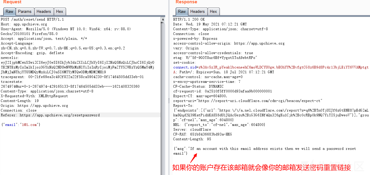
- 国外众测之密码找回漏洞
- 5g NR system messages
- Su embedded training - day4
猜你喜欢
How to learn a new technology (programming language)
Letcode43: string multiplication
Qt不同类之间建立信号槽,并传递参数
国外众测之密码找回漏洞

第四期SFO销毁,Starfish OS如何对SFO价值赋能?

Huawei switch s5735s-l24t4s-qa2 cannot be remotely accessed by telnet

Thinkphp内核工单系统源码商业开源版 多用户+多客服+短信+邮件通知

51与蓝牙模块通讯,51驱动蓝牙APP点灯
Where is the big data open source project, one-stop fully automated full life cycle operation and maintenance steward Chengying (background)?
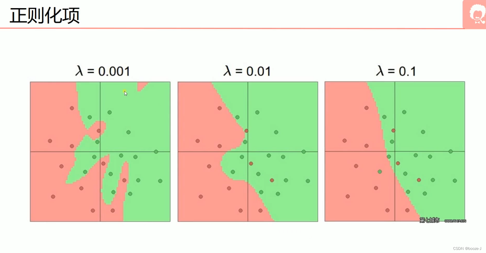
5.过拟合,dropout,正则化
随机推荐
New library launched | cnopendata China Time-honored enterprise directory
新库上线 | CnOpenData中国星级酒店数据
【obs】Impossible to find entrance point CreateDirect3D11DeviceFromDXGIDevice
Jemter distributed
接口测试进阶接口脚本使用—apipost(预/后执行脚本)
Play sonar
Stock account opening is free of charge. Is it safe to open an account on your mobile phone
服务器防御DDOS的方法,杭州高防IP段103.219.39.x
Leetcode brush questions
How to learn a new technology (programming language)
Huawei switch s5735s-l24t4s-qa2 cannot be remotely accessed by telnet
Marubeni official website applet configuration tutorial is coming (with detailed steps)
Handwriting a simulated reentrantlock
赞!idea 如何单窗口打开多个项目?
tourist的NTT模板
DNS series (I): why does the updated DNS record not take effect?
语义分割模型库segmentation_models_pytorch的详细使用介绍
Service Mesh的基本模式
22年秋招心得
RPA cloud computer, let RPA out of the box with unlimited computing power?