当前位置:网站首页>Cs231n notes (top) - applicable to 0 Foundation
Cs231n notes (top) - applicable to 0 Foundation
2022-07-05 15:55:00 【Small margin, rush】
This blog is Li Feifei :CS231n Before the computer vision course 13 Class notes
Catalog
k Proximity algorithm classifier ,k Is a super parameter
optimization - Find the gradient problem
Back propagation - Chain derivative
The first layer of visualization
Parameter by parameter adaptive learning rate method
Super parameter tuning - Random search is better than grid search
Image classification
Dataset training -> Given the image -> Judge , It should be robust

k Crossover verification : Analysis data set , Part of the training, part of the testing
k Proximity algorithm classifier ,k Is a super parameter
KNN The principle is when predicting a new value x When , According to the nearest K A point is what kind to judge x In which category .
Distance calculation : Harmanton 、 European style 、L1 distance /L2
k It's worth choosing : Select a smaller one through cross validation K Values start , Increasing K Value , Then calculate the variance of the validation set , Finally find a more suitable K value .
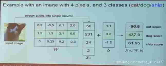
Linear classifier
f(xi,W,b)=Wxi+b
The linear classifier calculates 3 Matrix multiplication of the values and weights of all pixels in a color channel , So as to get the classification score .
According to the value we set for the weight , For certain colors at certain positions in the image , Functions that show a preference or dislike ( Depending on the sign of each weight ).
Loss function Loss function
The parameter of the scoring function is the weight matrix W, We can adjust the parameter of weight matrix , Make the scoring function in the correct classification position should get the highest score . Use the loss function to measure our dissatisfaction with the results . Directly speaking , When The greater the difference between the output result of the scoring function and the real result , The larger the loss function output , The smaller the vice .
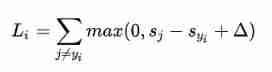
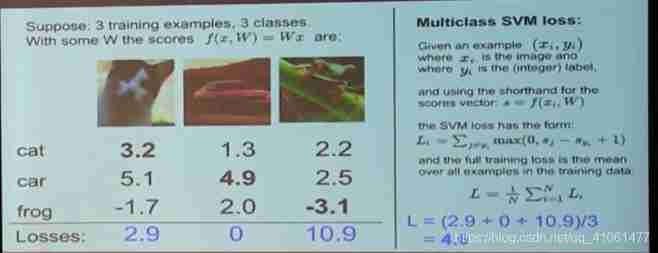
SVM Support vector machine loss
- SVM The loss function of wants SVM The score on the correct classification is always one boundary value higher than the score on the incorrect classification Δ
Regularization , Based on weights only
- Suppose there is a data set and a weight set W Be able to correctly classify each data ( There can be many similar W Can correctly classify all data ), When λ >1 when , Multiply any number by λW Can make the loss value 0
- We need to add another term to the original loss function Regularization term , The most common regularization term is L2 norm , It will impose a high penalty on the feature weight with a large range :
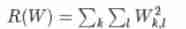
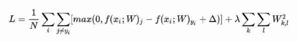
λ Is a super parameter , Cross validation is required to obtain ,N As the training set
About hyperparameters Δ : Hyperparameters Δ and λ It looks like two different super parameters , But they actually control the same trade-off together : That is, the trade-off between data loss and regularization loss in the loss function .
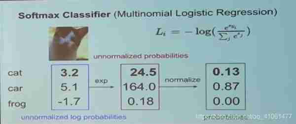
softmax classifier
Using cross entropy loss , The classification task is added to the last layer , Calculate the probability ( contrast svm Calculated value )
optimization - Find the gradient problem
Fine tune the slope in different dimensions , Traverse all of W.
mini-batch : A small batch of data is sampled in the data set to calculate the loss value , Fine tune parameters through back propagation
Back propagation - Chain derivative
Gate units communicate with each other through gradient signals , Just let their input change along the gradient , No matter how much their own output value rises or falls , To make the output value of the whole network higher .
The essence : Continuous partial derivative
In the whole calculation circuit diagram , Each gate cell gets some input and immediately calculates two things :1. The output value of this gate , and 2. The local gradient of the output value with respect to the input value . Once forward propagation is complete , In the process of back propagation , The gate unit gate will finally obtain the gradient of the final output value of the whole network on its own output value
neural network
Add nonlinear element , The formula is  , Parameters
  Will learn by random gradient descent .
Activation function
Each activation function ( Or nonlinear function ) The input of is a number , And then do some fixed mathematical operation on it .
- Sigmoid Nonlinear functions , Compress real numbers to [0,1] Between
- tanh function , Compress real numbers to [-1,1]
- ReLU It has a great accelerating effect on the convergence of random gradient descent , You need to set the learning rate
Neural network structure
Fully connected layer
The neurons in the whole connecting layer are completely connected in pairs with the neurons in the front and back layers , But there is no connection between neurons in the same fully connected layer
The forward propagation of the full connection layer is generally a matrix multiplication , Then add the offset and use the activation function .
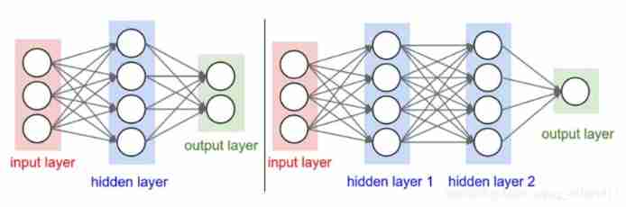
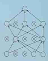
Determine the network size
- The first network has 4+2=6 Neurons ( Input layer not counted ),[3x4]+[4x2]=20 A weight , also 4+2=6 A bias , common 26 A learnable parameter .
- The second network has 4+4+1=9 Neurons ,[3x4]+[4x4]+[4x1]=32 A weight ,4+4+1=9 A bias , common 41 A learnable parameter .
Output layer
Neurons in the output layer generally do not have an activation function , The last output layer is mostly used to represent the classification score value , So it's a real number with any value , Or the target number of some real value
Set the number and size of layers
Neural networks with more neurons can express more complex functions , More complex data can be classified , The deficiency is that it may cause over fitting of training data .( Regularization techniques can be used to control over fitting )
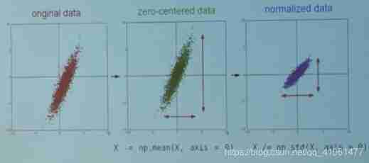
Data preprocessing
- Mean subtraction (Mean subtraction) It is independent of each other in the data features Minus the average
- normalization (Normalization) It refers to normalizing all dimensions of data , Make their numerical ranges approximately equal .( In image processing , Because the numerical range of pixels is almost the same ( All in 0-255 Between ))
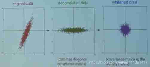
- PCA And albinism (Whitening) First, zero centralize the data , Then calculate the covariance matrix , It shows the correlation structure in the data . The input of the whitening operation is the data on the feature datum , Then each dimension is divided by its eigenvalue to normalize the range of values .
It should be divided into training / verification / Test set , Just average the pictures from the training set , Then each episode ( Training / verification / Test set ) Subtract this average from the image in .
The recommended preprocessing operation is to zero center each feature of the data , Then normalize the numerical range to [-1,1] Within limits .
The standard deviation used is
Gaussian distribution to initialize the weight , among n Is the number of neurons input . For example numpy Can write :w = np.random.randn(n) * sqrt(2.0/n).
 Gaussian distribution to initialize the weight , among n Is the number of neurons input . For example numpy Can write :w = np.random.randn(n) * sqrt(2.0/n).
Batch of normalization (Batch Normalization)
The method is to let the activation data pass through a network before the training starts , The network processes the data to make it obey the standard Gaussian distribution .
Regularization Regularization- By controlling the capacity of the neural network to prevent its over fitting
L1,L2, Maximum normal form constraint
Dropout: When it comes to forward propagation , Let the activation value of a neuron have a certain probability p Stop working , Make the generalization of the model stronger
Gradient check
- Use the centralization formula

- Use relative error
- Use double precision

The first layer of visualization
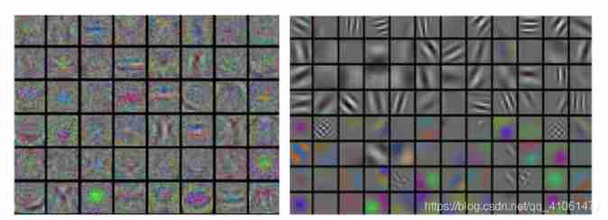
An example of visualizing the weights of the first layer of neural network . On the left The features in are full of noise , This suggests that there may be a problem with the network : The network does not converge , The learning rate is not set properly , The weight of regularization penalty is too low . Right picture It has good characteristics , smooth , Clean and diverse , It shows that the training process is well done .
Parameters are updated
Use back propagation to calculate analytical gradients , Gradient can be used to update parameters , The simplest form of updating is to change the parameters along the negative gradient ( Because the gradient points in the upward direction , But we usually want to minimize the loss function )
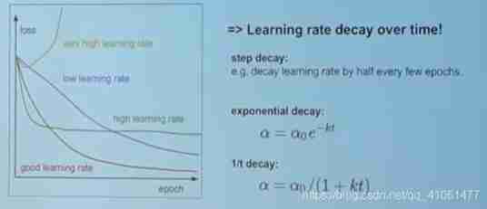
Learning rate -dropout
When training deep networks , Annealing the learning rate over time is usually helpful . If the learning rate is high , The kinetic energy of the system is too large , The parameter vector will jump irregularly , Can not be stabilized to the deeper and narrower part of the loss function .
Parameter by parameter adaptive learning rate method
The two recommended update methods are SGD+Nesterov Momentum method , perhaps Adam Method .
Super parameter tuning - Random search is better than grid search
Use random search ( Do not use grid search ) To search for the optimal hyperparameter . In stages from rough ( A wide range of training parameters 1-5 A cycle ) To fine ( There are many cycles of narrow range training ) To search .
Model integration
In practice , There is always a way to improve the accuracy of neural networks by a few percentage points , It is to train several independent models during training , Then average their predicted results during the test .
边栏推荐
- Data communication foundation NAT network address translation
- Noi / 1.4 07: collect bottle caps to win awards
- Bubble sort, insert sort
- episodic和batch的定义
- Appium自动化测试基础 — APPium基础操作API(一)
- JS knowledge points-01
- How to introduce devsecops into enterprises?
- Anti shake and throttling
- 力扣今日题-729. 我的日程安排表 I
- Hongmeng system -- Analysis from the perspective of business
猜你喜欢
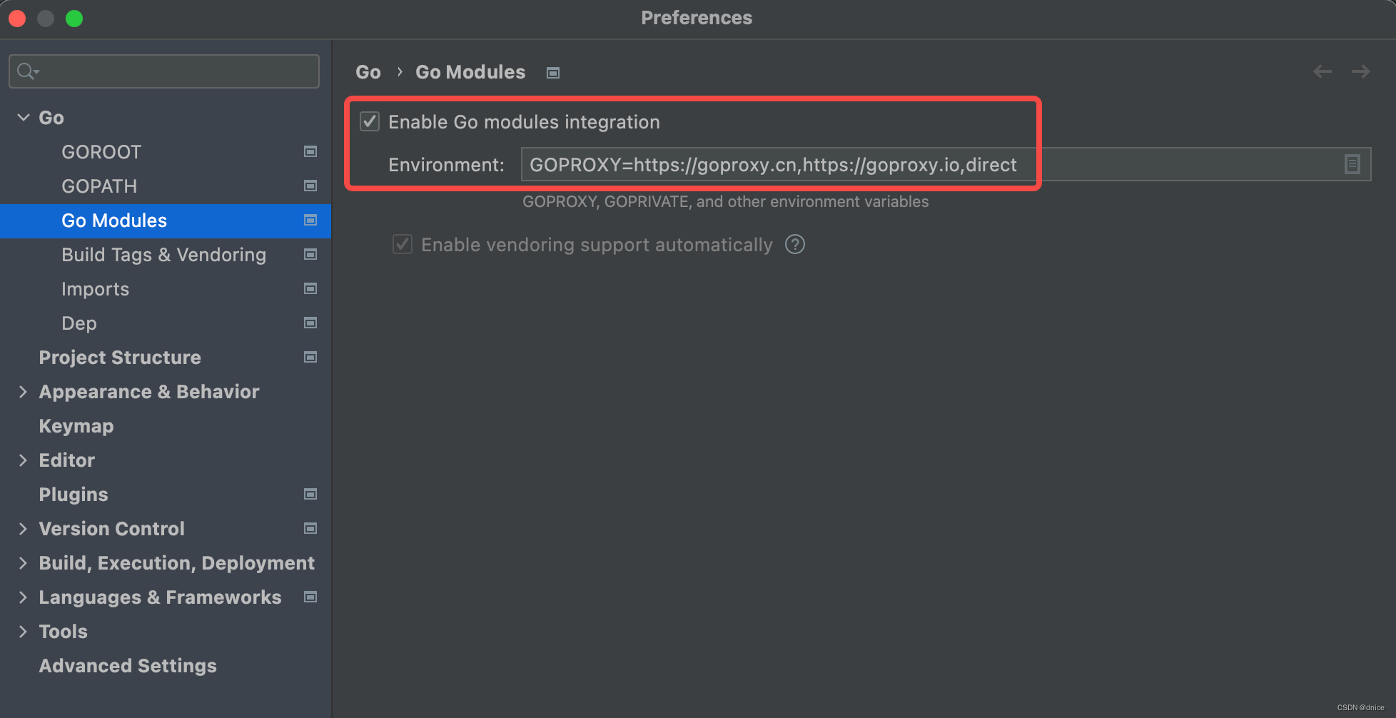
【簡記】解决IDE golang 代碼飄紅報錯

Object. defineProperty() - VS - new Proxy()

Write a go program with vscode in one article
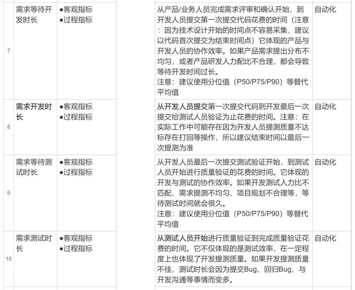
研发效能度量指标构成及效能度量方法论

CODING DevSecOps 助力金融企业跑出数字加速度
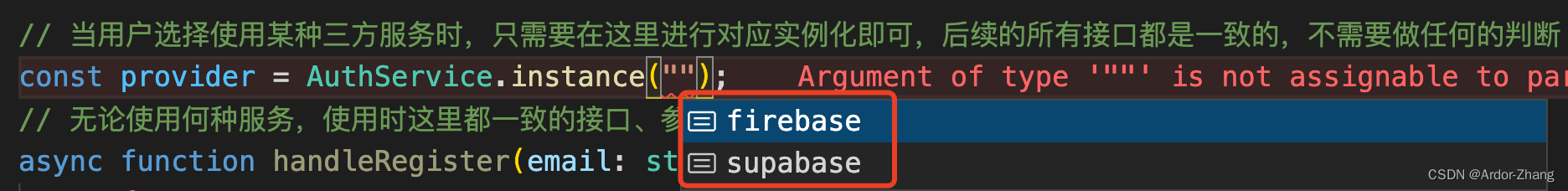
Transfer the idea of "Zhongtai" to the code
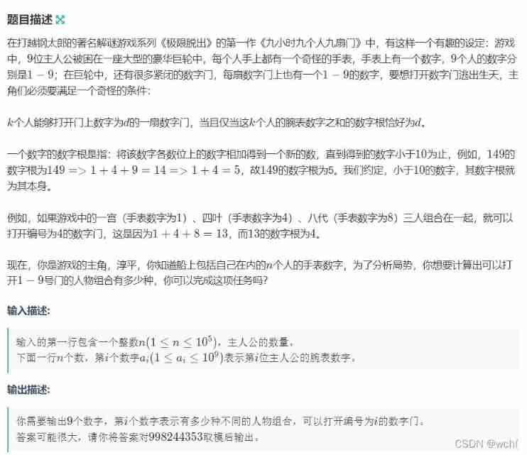
Nine hours, nine people, nine doors problem solving Report
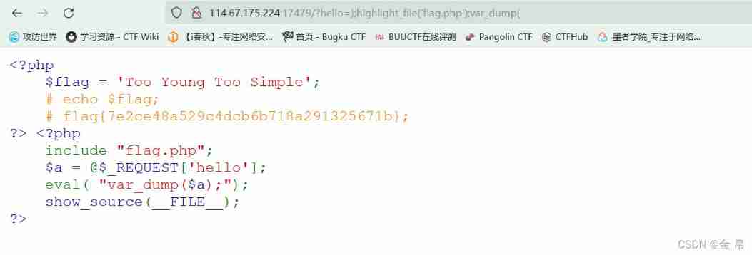
Bugku's Eval

Bugku's eyes are not real
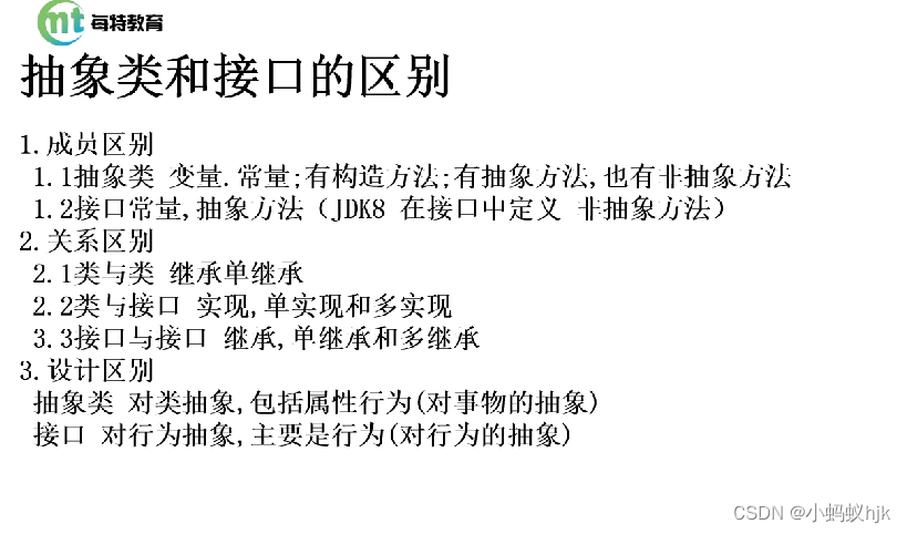
抽象类和接口的区别
随机推荐
机械臂速成小指南(九):正运动学分析
Data communication foundation OSPF Foundation
【簡記】解决IDE golang 代碼飄紅報錯
MySQL giant pit: update updates should be judged with caution by affecting the number of rows!!!
Five common negotiation strategies of consulting companies and how to safeguard their own interests
vant popup+其他组件的组合使用,及避坑指南
Go language programming specification combing summary
sql中查询最近一条记录
Bugku's Ping
Virtual base class (a little difficult)
vant tabbar遮挡内容的解决方式
go语言编程规范梳理总结
I spring and autumn blasting-1
This article takes you through the addition, deletion, modification and query of JS processing tree structure data
How difficult is it to pass the certification of Intel Evo 3.0? Yilian technology tells you
2.3 learning content
Clock switching with multiple relationship
一文带你吃透js处理树状结构数据的增删改查
Bugku's Eval
Appium automation test foundation - appium basic operation API (I)