Multilayer perceptron (pytorch)

https://courses.d2l.ai/zh-v2/

Multilayer perceptron

perceptron

• A given input $\mathbf{x}$, The weight $\mathbf{w}$, And offset b, Perceptron output ：
  $$o=\sigma (<w,x>+b)\sigma (x)=\{\begin{array}{l}1ifx>0\\ 0otherwise\end{array}$$

Perceptron is the problem of binary classification
hold 0 Change to -1 It's OK

• Two classification ：-1 or 1
  • Vs. Regression outputs real numbers
  • VS. Softmax Regression output probability

The output of linear regression is a real number , Here the output is a discrete class

Training perceptron

initalize w=0 and b=0
repeat
	if yi[<w,xi>+b] <= 0then	# <=0  It means that the perceptron predicts the sample incorrectly 
		w <-- w + yixi and b <-- b + yi
	end if
until all classfied correctly 

It's the multiplication of prediction and real value ,>0 The prediction is correct ,<0 Explain that the prediction is wrong .
If you don't understand it, you can learn the mathematical derivation of the perceptron first .

It is equivalent to using batch size of 1 The gradient of , And use the following loss function .
$$\theta (y,x,w)=max(0,-y<w,x>)$$

max Corresponding if sentence
When it's right ,loss by 0, Constant , There is no gradient
Be careful , Here, the learning rate of gradient descent is set to 1,

Convergence theorem

• The data is in the radius r Inside
• allowance $\rho$ There are two categories
  $$y(x^{T}w+b)\ge \rho$$
  about $||w|{|}^2+b^2\le 1$
• The sensor is guaranteed to be in $\frac{r^2+1}{{\rho }^2}$ Step by step convergence

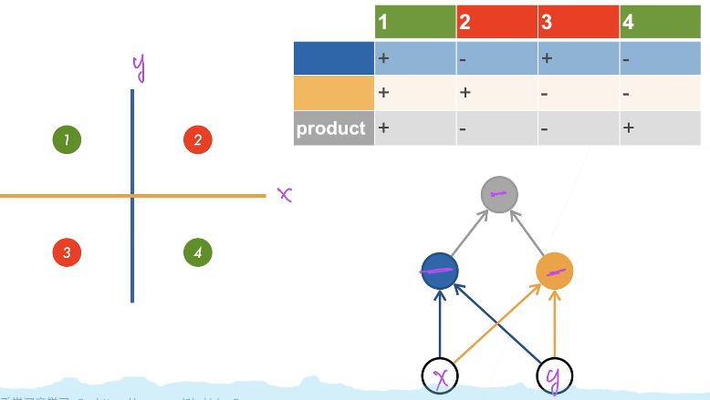
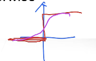
XOR problem （Minsky & Papert,1969）

The perceptron cannot fit XOR function , It can only produce linearly divided faces

summary

• Perceptron is a binary classification model , Is the earliest Al One of the models
• Its solution algorithm is equivalent to using a batch size of 1 The gradient of
• It cannot fit XOR function , For the first time Al The cold winter

Multilayer perceptron

Study XOR

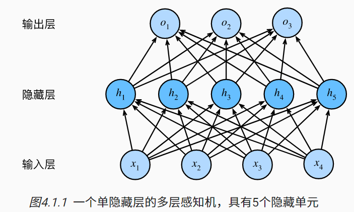
Single hidden layer

$$implicithiddenlayerBigSmallyessuperginsengCount$$

Single hidden layer — Single category

• Input $x\in R^n$
• Hidden layer $W_1\in R^{m\times n},b_1\in R^m$
• Output layer $w_2\in R^m,b_2\in R$
  $$\begin{gathered} h=\sigma (W_{1}x+b_1) \\ o=w_2^{T}h+b2 \end{gathered}$$

$\sigma$ Is the activation function by element

Why do we need a nonlinear activation function ？
Otherwise, the result is still the simplest linear function
hence $o=w_2^T{W}_{1}x+b^{\prime }$

Activation function

Sigmoid Activation function

Project input to （0,1）, It's a soft $\sigma (x)=\{\begin{array}{l}1ifx>0\\ 0otherwise\end{array}$

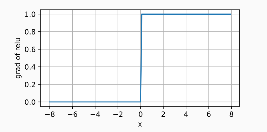
$\sigma (x)$ At the origin 0 It's hard to get derivative

$$sigmoid(x)=\frac{1}{1+exp(-x)}$$

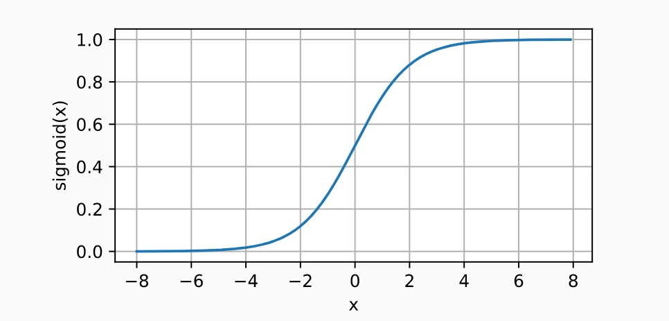
Tanh Activation function

Project input to （-1,1）
$$tanh(x)=\frac{1-exp(-2x)}{1+exp(-2x)}$$

ReLU Activation function

ReLU：rectified linear uint
$$ReLU(x)=max(x,0)$$

Deep learning is renaming many classic things

Multiple categories

$$y_1,y_2,...,y_k=softmax(o_1,o_2,...,o_k)$$

Multi class classification and softmax Return basically makes no difference , Is to add a hidden layer , Thus, it becomes a multi-layer perceptron
softmax Pull all input to 0 and 1 Region , So that they add up to 1, This gives the probability

• Input $x\in R^n$
• Hidden layer $W_1\in R^{m\times n},b_1\in R^m$
• Output layer $W_2\in R^{m\times k},b_2\in R^k$
  $$\begin{gathered} h=\sigma (W_{1}x+b_1) \\ o=W_2^{T}h+b2 \\ y=softmax(o) \end{gathered}$$

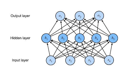
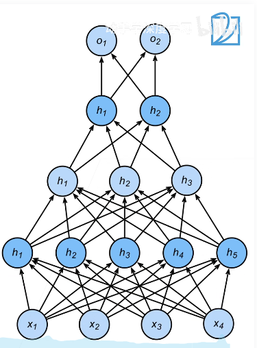
Multiple hidden layers

$$\begin{gathered} h_1=\sigma (W_{1}x+b_1) \\ {h}_2=\sigma (W_2{h}_1+b_2) \\ {h}_3=\sigma (W_3{h}_2+b_3) \\ o=W_4{h}_3+b_4 \end{gathered}$$

Hyperparameters

• Number of hidden layers
• The size of each hidden layer

The activation function is mainly used to avoid the collapse of layers
It means , If it is a linear mapping, all layers can be merged （ Collapse of layers ）, Nonlinearity cannot be merged

summary

• Multilayer perceptron uses hidden layer and activation function to obtain nonlinear model
• Commonly used activation functions Sigmoid,Tanh,ReLU
• Use Softmax To handle multi class classification
• The super parameter is the number of hidden layers , And the size of each hidden layer

The implementation of multi-layer perceptron starts from scratch

import torch
from torch import nn
from d2l import torch as d2l

batch_size = 256
train_iter, test_iter = d2l.load_data_fashion_mnist(batch_size)

Think about it ,Fashion-MNIST Each image in is represented by $28\times 28=784$ Composed of gray pixel values . All images are divided into 10 Categories . Ignore the spatial structure between pixels , We can think of each image as having 784 Input features and 10 A simple classification dataset of classes . First , We will implement a multi-layer perceptron with a single hidden layer , It contains 256 Hidden units . Be careful , We can treat both variables as hyperparameters . Usually , We choose 2 As the width of the layer . Because of the way memory is allocated and addressed in hardware , This tends to be computationally more efficient .

We use several tensors to represent our parameters . Be careful , For each layer, we need to record a weight matrix and an offset vector . Same as before , We need to allocate memory for the loss of gradients about these parameters .

num_inputs, num_outputs, num_hiddens = 784, 10, 256

W1 = nn.Parameter(torch.randn(
    num_inputs, num_hiddens, requires_grad=True) * 0.01)
b1 = nn.Parameter(torch.zeros(num_hiddens, requires_grad=True))
W2 = nn.Parameter(torch.randn(
    num_hiddens, num_outputs, requires_grad=True) * 0.01)
b2 = nn.Parameter(torch.zeros(num_outputs, requires_grad=True))

params = [W1, b1, W2, b2]

randn It's normal (0,1) Distribution , ride 0.01 Make the distribution normal (0,0.1) Distribution , The data variance is smaller .

Activation function

To make sure we know the details of the model like the back of our hand , We will achieve ReLU Activation function , Instead of calling the built-in relu function .

def relu(X):
    a = torch.zeros_like(X)
    return torch.max(X, a)

Model

Because we ignore the spatial structure , So we use reshape Convert each two-dimensional image into a length of num_inputs Vector . Our model can be implemented in just a few lines of code .

def net(X):
    X = X.reshape((-1, num_inputs))
    H = relu(X @ W1 + b1)  #  here “@” For matrix multiplication 
    return (H @ W2 + b2)

@ yes numpy Dot product operation symbol inside , amount to np.dot()

Loss function

Here we use advanced API The built-in function in the softmax And cross entropy loss .

loss = nn.CrossEntropyLoss(reduction='none')

Training

Fortunately, , The training process and of multi-layer perceptron softmax The training process for regression is exactly the same . Can be called directly d2l Bag train_ch3 function See Softmax Regression is achieved from scratch , Set the number of iteration cycles to 10, And set the learning rate to 0.1.

num_epochs, lr = 10, 0.1
updater = torch.optim.SGD(params, lr=lr)
d2l.train_ch3(net, train_iter, test_iter, loss, num_epochs, updater)

Simple implementation of multi-layer perceptron

We can pass the advanced API More concise implementation of multi-layer perceptron .

import torch
from torch import nn
from d2l import torch as d2l

Model

And softmax Compared with the concise implementation of regression , The only difference is that we added 2 All connection layers （ Before, we only added 1 All connection layers ）. The first layer is the hidden layer , It contains 256 Hidden units , And used ReLU Activation function . The second layer is the output layer .

net = nn.Sequential(nn.Flatten(),
                    nn.Linear(784, 256),
                    nn.ReLU(),
                    nn.Linear(256, 10))

def init_weights(m):
    if type(m) == nn.Linear:
        nn.init.normal_(m.weight, std=0.01)

net.apply(init_weights);

The realization of the training process is similar to our realization softmax Exactly the same when it comes back , This modular design enables us to separate the content related to the model architecture .

batch_size, lr, num_epochs = 256, 0.1, 10
loss = nn.CrossEntropyLoss(reduction='none')
trainer = torch.optim.SGD(net.parameters(), lr=lr)

train_iter, test_iter = d2l.load_data_fashion_mnist(batch_size)
d2l.train_ch3(net, train_iter, test_iter, loss, num_epochs, trainer)

• MLP(multi layer perceptron)( Multilayer perceptron ) If the effect is not good , Can be deconvoluted 、RNN、transformer
• If SVM( Support vector machine ) If you want more things

QA

1. What does a layer of neural network mean ？
   The so-called first floor , Generally speaking, it is weight 、 Add the activation function and your calculation
   It can be abbreviated as having several layers of weight W, Just how many floors
   Input layer is not a layer

2. SVM and MLP
   SVM Insensitive to super parameters , Optimization and adjustment will be easier
   Multilayer perceptron and SVM The effect is almost the same
   SVM Mathematical expressions are beautiful
   MLP It is easy to change to other neural networks

3. Why should neural networks increase the number of hidden layers , Not the number of neurons ？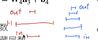

Theoretically , The model is about the same size
The right side is called deep learning , Good training
The left side is called shallow learning （ Width learning ）, Easy to overfit
You can't be a fat man at one bite ！

Teacher Li Hongyi spoke this piece very well