当前位置:网站首页>Tensorflow—Neural Style Transfer
Tensorflow—Neural Style Transfer
2022-07-03 10:27:00 【JallinRichel】
Style transfer [Style_transfer] Learning notes ——Tensorflow
- The actual effect of the tutorial is shown
- Overview of style transfer & The implementation idea of this tutorial
- Preparation
- Code implementation
- Thank you for watching !!!
explain : This article is for the author to learn Tensorflow Study notes during the official tutorial , Now it is sorted out for your reference . You can read and learn this article as the Chinese translation of the official tutorial . The code of this tutorial is consistent with the official code , There are only a few minor changes .
Tensorflow The official tutorial link is attached at the end of the article .
The actual effect of the tutorial is shown
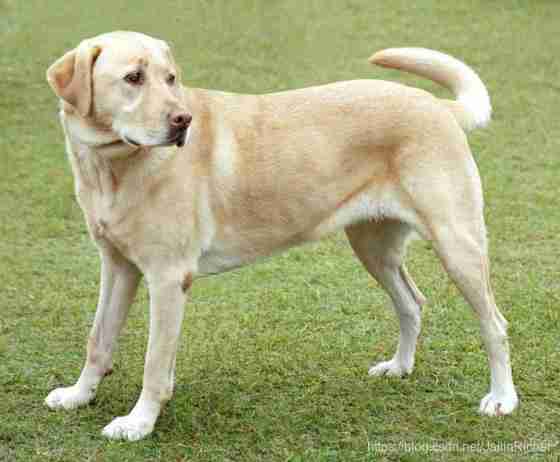
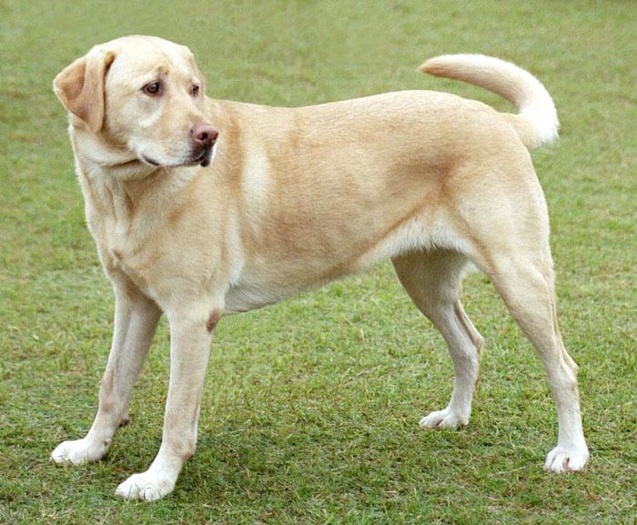
This tutorial will use pictures 1 With pictures 2 Generate pictures 3
picture 1—— Content picture 1
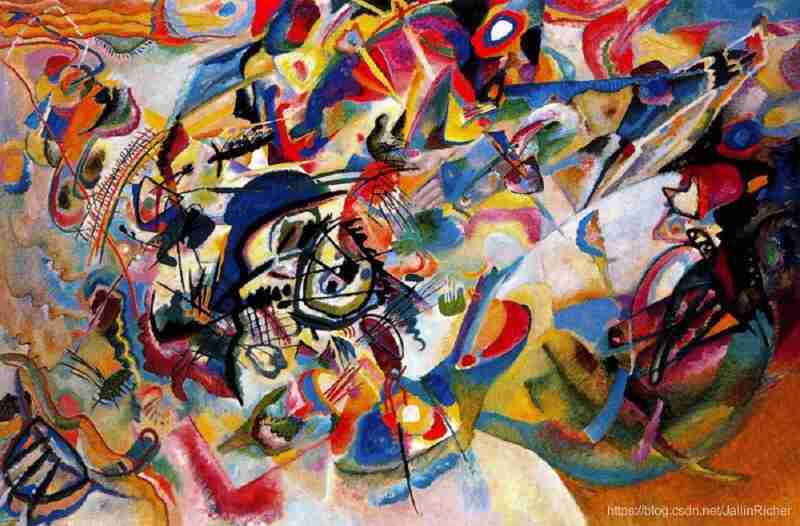
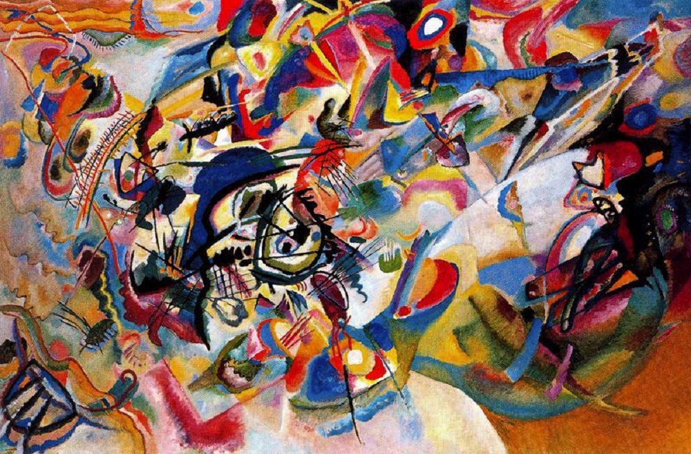
picture 2—— Style picture 2
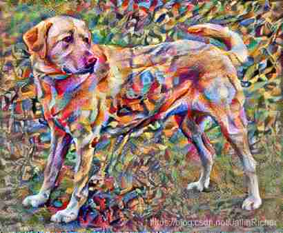
picture 3—— Result pictures ( Parameter setting epoch=10, step_per_epoch=100)
Overview of style transfer & The implementation idea of this tutorial
Overview of style transfer
The image passes by The covariance matrix of the feature map obtained after convolution layer can well characterize the texture features of the image , But it will lose location information . But in the task of style transfer , We can ignore the disadvantage of location information loss , Just find a way to represent the texture information of the image , And transfer these texture information to the image that needs to be transferred by style , Complete the task of style migration .
In this tutorial , We use Clem matrix instead of covariance matrix , It can describe the autocorrelation of global features .
The implementation idea of this tutorial
In this tutorial , We start from the trained image classification network VGG19 Select the middle layer to extract the texture features of the image .
The official tutorial also introduces the use of Tensorflow_Hub Examples of direct and rapid style migration , In this article, we will not repeat .
Preparation
Software preparation
- install anaconda The latest version 3, Click on Download Select the corresponding version to download ;( It is recommended to use GPU edition )
The author's CPU by Intel Core i5-8300H CPU @ 2.30GHz 2.30 GHz - This tutorial USES Python 3.7.7 edition
- install Tensorflow、Keras、Matplotlib、Numpy
Data preparation ( Download content and style pictures )
content_path = tf.keras.utils.get_file('YellowLabradorLooking_new.jpg', 'https://storage.googleapis.com/download.tensorflow.org/example_images/YellowLabradorLooking_new.jpg')
style_path = tf.keras.utils.get_file('kandinsky5.jpg','https://storage.googleapis.com/download.tensorflow.org/example_images/Vassily_Kandinsky%2C_1913_-_Composition_7.jpg')
Code implementation
Import corresponding modules
import os
import tensorflow as tf
# Load compressed models from tensorflow_hub
os.environ['TFHUB_MODEL_LOAD_FORMAT'] = 'COMPRESSED'

import IPython.display as display

import matplotlib.pyplot as plt
import matplotlib as mpl
mpl.rcParams['figure.figsize'] = (12, 12)
mpl.rcParams['axes.grid'] = False

import numpy as np
import PIL.Image
import time
import functools

def tensor_to_image(tensor): # Define the transformation function from tensor to image
  tensor = tensor*255
  tensor = np.array(tensor, dtype=np.uint8)
  if np.ndim(tensor)>3:
    assert tensor.shape[0] == 1
    tensor = tensor[0]
  return PIL.Image.fromarray(tensor)
Show on the screen that two pictures have been downloaded
- Define a function to load pictures , And limit the maximum size of the picture to 512 Pixels .
def load_img(path_to_img):
  max_dim = 512
  img = tf.io.read_file(path_to_img)
  img = tf.image.decode_image(img, channels=3)
  img = tf.image.convert_image_dtype(img, tf.float32)

  shape = tf.cast(tf.shape(img)[:-1], tf.float32)
  long_dim = max(shape)
  scale = max_dim / long_dim

  new_shape = tf.cast(shape * scale, tf.int32)

  img = tf.image.resize(img, new_shape)
  img = img[tf.newaxis, :]
  return img
- Define a function to display pictures
def imshow(image, title=None):
  if len(image.shape) > 3:
    image = tf.squeeze(image, axis=0)

  plt.imshow(image)
  if title:
    plt.title(title)
- Display images
content_image = load_img(content_path)
style_image = load_img(style_path)

plt.subplot(1, 2, 1)
imshow(content_image, 'Content Image')

plt.subplot(1, 2, 2)
imshow(style_image, 'Style Image')
Now two pictures should be displayed on your screen 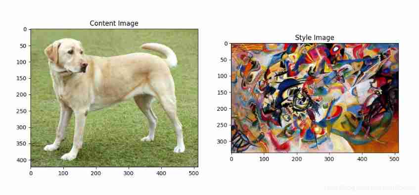
Define content and style expression
We can use the middle layer of the model to obtain the content and style of the image .
Start with the input layer of the network , The first few layers can be used to represent low-level features such as edges and textures . When you browse the Internet step by step , The last few layers can be used to represent the high-level features of the image —— Such as wheels or eyes .
In this tutorial , We use VGG19 The middle layer of the network architecture defines the content and style of the image , Try to match the corresponding style and content target representation on these middle layers .
- Load a that does not contain a classification header VGG19, List its layer name
vgg = tf.keras.applications.VGG19(include_top=False, weights='imagenet')
# If you want to load the classification header , You can take the top one  False Change it to  True
print()
for layer in vgg.layers:
  print(layer.name)
- Choose the middle tier from the network to express the content and style of the picture
content_layers = ['block5_conv2']

style_layers = ['block1_conv1',
                'block2_conv1',
                'block3_conv1',
                'block4_conv1',
                'block5_conv1']

num_content_layers = len(content_layers)
num_style_layers = len(style_layers)
Why can these intermediate output layers define the content and style representation of pictures
In high-level features , A network wants to realize image classification , Then it must understand the picture . This requires the original image as the input pixel , And create an internal representation , The complex understanding of converting the original image pixels into the corresponding image features .
This is also one reason why convolutional neural network can have better results : They can capture the invariance and defining features of classes that are not affected by background noise and other disturbances .
So when the image is input into the model , At this time, the model acts as a complex feature extractor . By accessing the middle tier of the model , We can describe the content and style of the input image .
Build a model
- The network is designed in tf.keras.applications in , We can go through Keras functional API Extract the value of the middle layer .
- We can use model = Model(inputs, outputs) To define the model .
The following function can build a VGG19 Model
def vgg_layers(layer_names):
  """ Creates a vgg model that returns a list of intermediate output values."""
  # Load our model. Load pretrained VGG, trained on imagenet data
  vgg = tf.keras.applications.VGG19(include_top=False, weights='imagenet')
  vgg.trainable = False

  outputs = [vgg.get_layer(name).output for name in layer_names]

  model = tf.keras.Model([vgg.input], outputs)
  return model

style_extractor = vgg_layers(style_layers)
style_outputs = style_extractor(style_image*255)

#Look at the statistics of each layer's output
for name, output in zip(style_layers, style_outputs):
  print(name)
  print(" shape: ", output.numpy().shape)
  print(" min: ", output.numpy().min())
  print(" max: ", output.numpy().max())
  print(" mean: ", output.numpy().mean())
  print()
Computing style ( Calculate the Clem matrix )
By taking the outer product of the eigenvector and itself at each position , And find the average value of the outer product at all positions , Calculate the Clem matrix containing this information .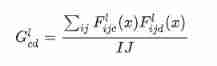
This can be used tf.linalg.einsum Function to implement
def gram_matrix(input_tensor):
  result = tf.linalg.einsum('bijc,bijd->bcd', input_tensor, input_tensor)
  input_shape = tf.shape(input_tensor)
  num_locations = tf.cast(input_shape[1]*input_shape[2], tf.float32)
  return result/(num_locations)
Extract the style and content of the image
Build a model of return style and content tensor
class StyleContentModel(tf.keras.models.Model):
  def __init__(self, style_layers, content_layers):
    super(StyleContentModel, self).__init__()
    self.vgg = vgg_layers(style_layers + content_layers)
    self.style_layers = style_layers
    self.content_layers = content_layers
    self.num_style_layers = len(style_layers)
    self.vgg.trainable = False

  def call(self, inputs):
    "Expects float input in [0,1]"
    inputs = inputs*255.0
    preprocessed_input = tf.keras.applications.vgg19.preprocess_input(inputs)
    outputs = self.vgg(preprocessed_input)
    style_outputs, content_outputs = (outputs[:self.num_style_layers],
                                      outputs[self.num_style_layers:])

    style_outputs = [gram_matrix(style_output)
                     for style_output in style_outputs]

    content_dict = {
    content_name: value
                    for content_name, value
                    in zip(self.content_layers, content_outputs)}

    style_dict = {
    style_name: value
                  for style_name, value
                  in zip(self.style_layers, style_outputs)}

    return {
    'content': content_dict, 'style': style_dict}

extractor = StyleContentModel(style_layers, content_layers)

results = extractor(tf.constant(content_image))
When we input the image , The model will return style_layers Clem matrix and content_layers The content of .
The operating gradient drops
With style and content extractors , We can now run the style migration algorithm program .
By calculating the mean square error of the image output relative to each target , Then take the weighted sum of these losses .
Establish style and content goals
style_targets = extractor(style_image)['style']
content_targets = extractor(content_image)['content']
Define a tf.Variable To include the image to be optimized . In the code before the article, the pixel value of the image has been set to float32 type .(tf.Variable Must have the same shape as the content image )
In order to make the algorithm faster , We limit the pixel value of the picture to 0 To 1 Between
image = tf.Variable(content_image)

def clip_0_1(image):
  return tf.clip_by_value(image, clip_value_min=0.0, clip_value_max=1.0)
Build an optimizer , And use the weighted combination of the two losses to get the total loss .
When used in this tutorial Adma, But recommended LBFGS.
opt = tf.optimizers.Adam(learning_rate=0.02, beta_1=0.99, epsilon=1e-1)

style_weight=1e-2
content_weight=1e4

def style_content_loss(outputs):
    style_outputs = outputs['style']
    content_outputs = outputs['content']
    style_loss = tf.add_n([tf.reduce_mean((style_outputs[name]-style_targets[name])**2)
                           for name in style_outputs.keys()])
    style_loss *= style_weight / num_style_layers

    content_loss = tf.add_n([tf.reduce_mean((content_outputs[name]-content_targets[name])**2)
                             for name in content_outputs.keys()])
    content_loss *= content_weight / num_content_layers
    loss = style_loss + content_loss
    return loss
Use tf,GradientTape To update the picture
@tf.function()
def train_step(image):
  with tf.GradientTape() as tape:
    outputs = extractor(image)
    loss = style_content_loss(outputs)

  grad = tape.gradient(loss, image)
  opt.apply_gradients([(grad, image)])
  image.assign(clip_0_1(image))
Now we can try to run our program several times
train_step(image)
train_step(image)
train_step(image)
tensor_to_image(image)
Output results :

Then we run it many times , For better results
import time
start = time.time()

epochs = 10
steps_per_epoch = 100

step = 0
for n in range(epochs):
  for m in range(steps_per_epoch):
    step += 1
    train_step(image)
    print(".", end='', flush=True)
  display.clear_output(wait=True)
  display.display(tensor_to_image(image))
  print("Train step: {}".format(step))

end = time.time()
print("Total time: {:.1f}".format(end-start))
If the reader who carries out this step uses CPU Version! , The speed of producing results will be relatively slow , Can be epochs perhaps step_per_epoch Set the value of lower .
Output results :
- This tutorial ends here , In the official course 4 There are subsequent optimizations in , Interested readers can click on the link below .
Thank you for watching !!!
边栏推荐
- ECMAScript -- "ES6 syntax specification # Day1
- Yolov5 creates and trains its own data set to realize mask wearing detection
- [LZY learning notes dive into deep learning] 3.1-3.3 principle and implementation of linear regression
- Hands on deep learning pytorch version exercise solution - 2.6 probability
- LeetCode - 673. Number of longest increasing subsequences
- CV learning notes - edge extraction
- LeetCode - 706 设计哈希映射(设计) *
- 波士顿房价预测(TensorFlow2.9实践)
- Opencv image rotation
- 20220610其他:任务调度器
猜你喜欢

LeetCode - 933 最近的请求次数
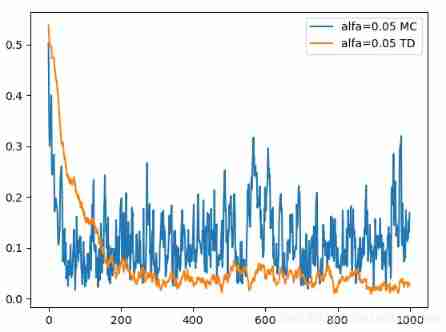
4.1 Temporal Differential of one step
LeetCode - 1670 設計前中後隊列(設計 - 兩個雙端隊列)
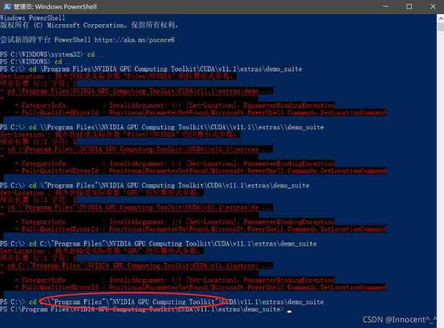
Powshell's set location: unable to find a solution to the problem of accepting actual parameters

Leetcode 300 longest ascending subsequence
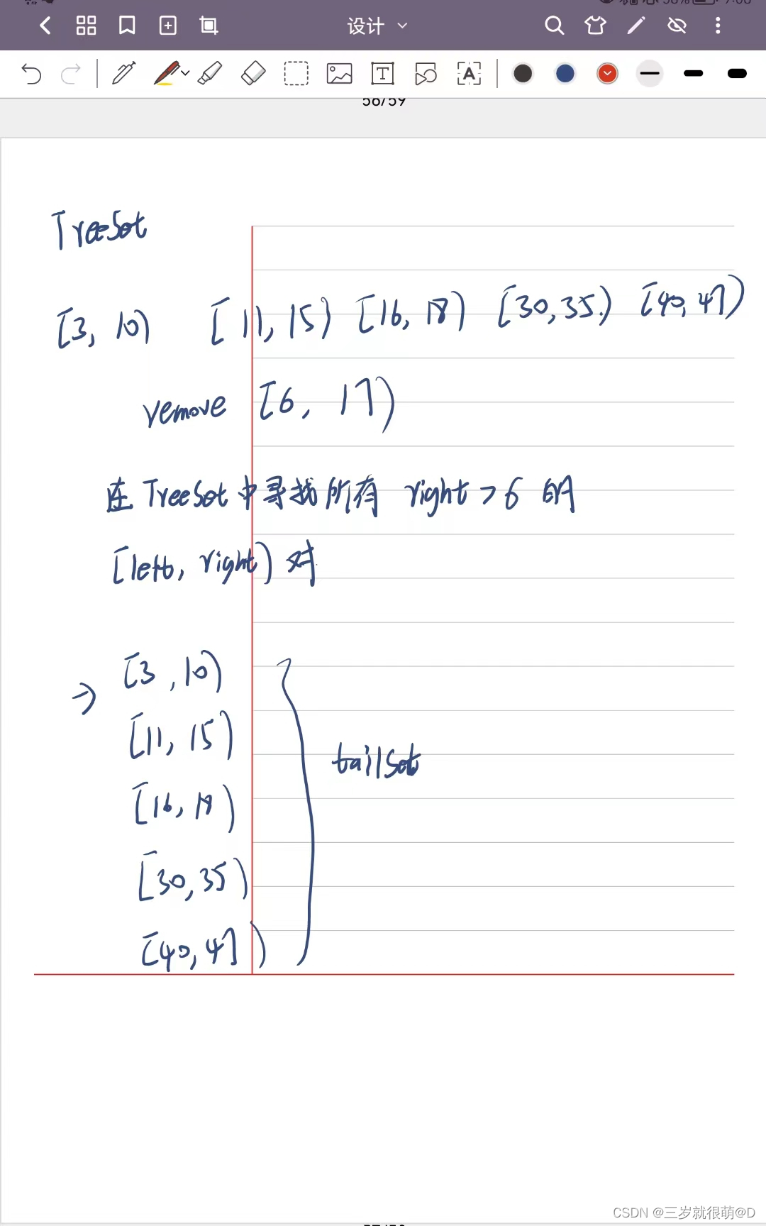
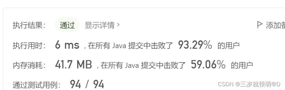
LeetCode - 715. Range module (TreeSet)*****

CV learning notes - clustering
Opencv Harris corner detection

Connect Alibaba cloud servers in the form of key pairs
『快速入门electron』之实现窗口拖拽
随机推荐
Data classification: support vector machine
Opencv notes 17 template matching
I really want to be a girl. The first step of programming is to wear women's clothes
20220601数学:阶乘后的零
Leetcode-513: find the lower left corner value of the tree
Codeup: word replacement
Opencv gray histogram, histogram specification
Hands on deep learning pytorch version exercise solution - 3.1 linear regression
Markdown latex full quantifier and existential quantifier (for all, existential)
侯捷——STL源码剖析 笔记
Leetcode-404:左叶子之和
Leetcode - the k-th element in 703 data flow (design priority queue)
Deep Reinforcement learning with PyTorch
LeetCode - 919. Full binary tree inserter (array)
2018 y7000 upgrade hard disk + migrate and upgrade black apple
[LZY learning notes dive into deep learning] 3.4 3.6 3.7 softmax principle and Implementation
Leetcode - 1670 design front, middle and rear queues (Design - two double ended queues)
20220603 Mathematics: pow (x, n)
Hands on deep learning pytorch version exercise solution - 2.4 calculus
Yolov5 creates and trains its own data set to realize mask wearing detection