当前位置:网站首页>Nonlinear optimization: establishment of slam model
Nonlinear optimization: establishment of slam model
2022-07-02 10:18:00 【Jason. Li_ 0012】
SLAM mathematical model
Equation of motion
Set the robot in the process of driving , moment t t t The pose of is x t x_t xt, Then the motion equation of the robot can be expressed by the following formula :
x k = f ( x k − 1 , u k , w k ) x_k=f(x_{k-1},u_k,w_k) xk=f(xk−1,uk,wk)
among , u k u_k uk It is the control quantity, that is, the reading or input of the motion sensor . Generally, the encoder is used to obtain the travel speed of the robot ( Speed motion model ) Or use odometer to obtain mileage information ( Mileage model ) As input . w k w_k wk Is the motion noise item .
The meaning of the equation of motion is , Through the position and posture information and control quantity of the robot at the last moment , It can estimate the current position and posture of the robot .
The observation equation
Vision SLAM The observation model of is usually a feature-based model , Then the map information is composed of some columns of road signs . use y 1 , y 2 , ⋯ , y N y_1,y_2,\cdots,y_N y1,y2,⋯,yN It indicates each road punctuation .
In the process of robot movement , The sensor will get the information of the surrounding road signs , Then the observation equation of the robot is as follows :
z k , j = h ( y j , x k , v k , j ) z_{k,j}=h(y_j,x_k,v_{k,j}) zk,j=h(yj,xk,vk,j)
among , v k , j v_{k,j} vk,j Is the observation noise item .
The meaning of observation equation is , In the road sign information y j y_j yj And robot posture x k x_k xk Next , The observation data of the sensor is z k , j z_{k,j} zk,j
State estimation problem
thus , obtain SLAM Model of :
{ x k = f ( x k − 1 , u k , w k ) z k , j = h ( y j , x k , v k , j ) \begin{cases}x_k=f(x_{k-1},u_k,w_k)\\z_{k,j}=h(y_j,x_k,v_{k,j})\end{cases} { xk=f(xk−1,uk,wk)zk,j=h(yj,xk,vk,j)
among , The current pose of the robot in the equation of motion x k x_k xk May by T k ∈ S E ( 3 ) T_k\in SE(3) Tk∈SE(3) Describe . The observation equation is modeled by the camera pinhole model :
s z k , j = K ( R k y j + t k ) s\:z_{k,j}=K(R_{k}y_j+t_k) szk,j=K(Rkyj+tk)
That is, at the moment t t t Next , The camera sensor is in the robot position x k x_k xk It's about , At this time, the road signs y j y_j yj The observation made corresponds to the pixel position on the image z k , j z_{k,j} zk,j It's about . among , s s s Is the scale factor , K K K For camera internal reference , R k ∈ S O ( 3 ) R_k\in SO(3) Rk∈SO(3) Move peacefully t k t_k tk It forms the external parameter matrix of the camera T k T_k Tk.
Usually , Increase with zero as the mean R k 、 Q k , j R_k、Q_{k,j} Rk、Qk,j Is the Gaussian distribution of variance w k , v k , j w_k,v_{k,j} wk,vk,j As motion noise and observation noise :
w k ∼ N ( 0 , R k ) v k , j ∼ N ( 0 , Q k , j ) w_k\sim \mathcal{N}(0,R_k)\qquad\qquad v_{k,j}\sim \mathcal{N}(0,Q_{k,j}) wk∼N(0,Rk)vk,j∼N(0,Qk,j)
According to the model , Adopt control quantity u u u( Usually speed information or odometer information ) And sensor observation z z z Infer the pose of the robot x x x And map information y y y
There are two ways to deal with the problem of state estimation , One is called filter algorithm , One is batch Estimation Algorithm . The filter algorithm holds an estimate of the current moment , And update the estimation with new sensor data . The batch estimation calculation method accumulates the data into a small batch , Unified processing and estimation .
The commonly used filter algorithm is extended Kalman Algorithm (EKF)、 Unscented Kalman Algorithm (UKF) etc. . Relatively speaking , The filter algorithm only cares about the state estimator at the current moment , The batch estimation is optimized in a larger range . It is generally believed that batch estimation is better than filter estimation .
Batch estimation
For robot motion , Consider from 1 To N The position and posture of the robot at any time x t x_t xt And the corresponding landmark information y j y_j yj:
x = { x 1 , ⋯ , x N } y = { y 1 , ⋯ , y M } x=\{x_1,\cdots,x_N\}\qquad\qquad y=\{y_1,\cdots,y_M\} x={ x1,⋯,xN}y={ y1,⋯,yM}
Then input u u u、 Sensor observation data z z z The robot shape is estimated as follows under the condition of :
p ( x , y ∣ z , u ) = p ( z , u ∣ x , y ) p ( x , y ) p ( z , u ) = η p ( z , u ∣ x , y ) p ( x , y ) p(x,y|z,u)=\frac{p(z,u|x,y)\:p(x,y)}{p(z,u)}=\eta\:p(z,u|x,y)\:p(x,y) p(x,y∣z,u)=p(z,u)p(z,u∣x,y)p(x,y)=ηp(z,u∣x,y)p(x,y)
Bayesian law unfolds , Get the content on the right , among η \eta η Is the normalization factor ; p ( z , u ∣ x , y ) p(z,u|x,y) p(z,u∣x,y) by likelihood (Likehood); p ( x , y ) p(x,y) p(x,y) by transcendental (Prior); p ( x , y ∣ z , u ) p(x,y|z,u) p(x,y∣z,u) by Posttest .
It is difficult to solve the posterior distribution directly , Turn to solving an optimal state estimation , Maximize the posterior probability :
( x , y ) M A P ∗ = a r g max p ( x , y ∣ z , u ) = a r g max p ( z , u ∣ x , y ) p ( x , y ) (x,y)^*_{MAP}=arg\max\:p(x,y|z,u)=arg\max\:p(z,u|x,y)p(x,y) (x,y)MAP∗=argmaxp(x,y∣z,u)=argmaxp(z,u∣x,y)p(x,y)
Normalization factor η \eta η Independent of distribution , Classified as a constant term , Ignore . From the above equation : To maximize the posterior probability is to solve the most Large likelihood estimation :
( x , y ) M L E ∗ = a r g max p ( z , u ∣ x , y ) (x,y)^*_{MLE}=arg\max\:p(z,u|x,y) (x,y)MLE∗=argmaxp(z,u∣x,y)
Likelihood means : Under the current robot posture , Possible observational data .
Maximum likelihood estimation : In what state does the robot pose , Most likely to get the currently observed data .
Maximum likelihood estimation
Observation model
( x , y ) M L E ∗ = a r g m a x p ( z , u ∣ x , y ) (x,y)^*_{MLE}=arg\:max\:p(z,u|x,y) (x,y)MLE∗=argmaxp(z,u∣x,y)
For an observation :
z k , j = h ( y j , x k ) + v k , j z_{k,j}=h(y_j,x_k)+v_{k,j} zk,j=h(yj,xk)+vk,j
Modeling observation noise with Gaussian distribution v t , j ∼ N ( 0 , Q k , j ) v_{t,j}\sim\mathcal{N}(0,Q_{k,j}) vt,j∼N(0,Qk,j), Then we can see :
p ( z k , j ∣ x k , y j ) ∼ N ( h ( y j , x k ) , Q k , j ) p(z_{k,j}|x_k,y_j)\sim\mathcal{N}(h(y_j,x_k),Q_{k,j}) p(zk,j∣xk,yj)∼N(h(yj,xk),Qk,j)
To solve the maximum likelihood estimation, you can use Minimize the negative logarithm In a way that .
Minimum negative logarithm
For an arbitrary high latitude Gaussian distribution x ∼ N ( μ , Σ ) x\sim\mathcal{N}(\mu,\Sigma) x∼N(μ,Σ):
p ( x ) = 1 ( 2 π ) N d e t ( Σ ) e x p ( − 1 2 ( x − μ ) T Σ − 1 ( x − μ ) ) p(x)=\frac{1}{\sqrt{(2\pi)^Ndet(\Sigma)}}exp\Bigl(-\frac{1}{2}(x-\mu)^T\Sigma^{-1}(x-\mu)\Bigr) p(x)=(2π)Ndet(Σ)1exp(−21(x−μ)TΣ−1(x−μ))
Take the negative natural logarithm :
− ln p ( x ) = 1 2 ln ( ( 2 π ) N d e t ( Σ ) ) + 1 2 ( x − μ ) T Σ − 1 ( x − μ ) -\ln\:p(x)=\frac{1}{2}\ln\Bigl((2\pi)^N\:det(\Sigma)\Bigr)+\frac{1}{2}(x-\mu)^T\Sigma^{-1}(x-\mu) −lnp(x)=21ln((2π)Ndet(Σ))+21(x−μ)TΣ−1(x−μ)
Monotonically increasing property of logarithmic function , You can get right p ( x ) p(x) p(x) Find the maximization, that is, the negative logarithm − ln p ( x ) -\ln\:p(x) −lnp(x) Minimize .
The first term on the right of the above expression is a constant term , Then the maximum likelihood estimation of the state can be obtained by solving the minimum term of the second term on the right .
Maximum likelihood estimation
Bring the observation equation into the above model :
( x k , y j ) ∗ = a r g max N ( h ( y j , x k ) , Q k , j ) = a r g min ( ( z k , j − h ( x k , y j ) ) T Q k , j − 1 ( z k , j − h ( x k , y j ) ) ) \begin{aligned} (x_k,y_j)^*& =arg\max\:\mathcal{N}(h(y_j,x_k),Q_{k,j})\\ &=arg\min\Bigl(\bigl(z_{k,j}-h(x_k,y_j)\bigr)^TQ_{k,j}^{-1}\bigl(z_{k,j}-h(x_k,y_j)\bigr)\Bigr)\\ \end{aligned} (xk,yj)∗=argmaxN(h(yj,xk),Qk,j)=argmin((zk,j−h(xk,yj))TQk,j−1(zk,j−h(xk,yj)))
Call the mahalanobi distance described by the above formula , Mahalanobis distance . The expression is equivalent to minimizing the noise term , Q k , j − 1 Q_{k,j}^{-1} Qk,j−1 It is called information matrix , That is, the inverse of the covariance matrix of Gaussian distribution .
Batch estimation
Consider the data at the time of batch , Suppose the control quantity input at each time in the batch u u u、 Sensor observation data z z z Are independent of each other , That is, the control quantities are independent of each other , The observations are independent of each other , Available :
p ( z , u ∣ x , y ) = ∏ k p ( u k ∣ x k − 1 , x k ) ∏ k , j p ( z k , j ∣ x k , y j ) p(z,u|x,y)=\prod_kp(u_k|x_{k-1},x_k)\:\prod_{k,j}p(z_{k,j}|x_k,y_j) p(z,u∣x,y)=k∏p(uk∣xk−1,xk)k,j∏p(zk,j∣xk,yj)
thus , It can independently handle the movement at all times 、 observation . Now define the motion control quantity 、 The errors between the sensor observation and the model are as follows :
e u , k = x k − f ( x k − 1 , u k ) e z , k , j = z k , j − h ( x k , y j ) \begin{aligned} e_{u,k}&=x_k-f(x_{k-1},u_k)\\ e_{z,k,j}&=z_{k,j}-h(x_k,y_j)\\ \end{aligned} eu,kez,k,j=xk−f(xk−1,uk)=zk,j−h(xk,yj)
thus , The objective function is as follows :
min J ( x , y ) = ∑ k e u , k T R k − 1 e u , k + ∑ k ∑ j e z , k , j T Q k , j − 1 e z , k , j \min J(x,y)=\sum_ke_{u,k}^TR_k^{-1}e_{u,k}+\sum_k\sum_je_{z,k,j}^TQ_{k,j}^{-1}e_{z,k,j} minJ(x,y)=k∑eu,kTRk−1eu,k+k∑j∑ez,k,jTQk,j−1ez,k,j
here , In practice, the minimum negative logarithm is used to solve the maximum likelihood estimation problem , Therefore, the cumulative multiplication becomes cumulative in the form of negative logarithm .
Minimize the objective function to nonlinear The least squares problem .
边栏推荐
- [unreal] animation notes of the scene
- C language strawberry
- Operator exercises
- 【Unity3D】无法正确获取RectTransform的属性值导致计算出错
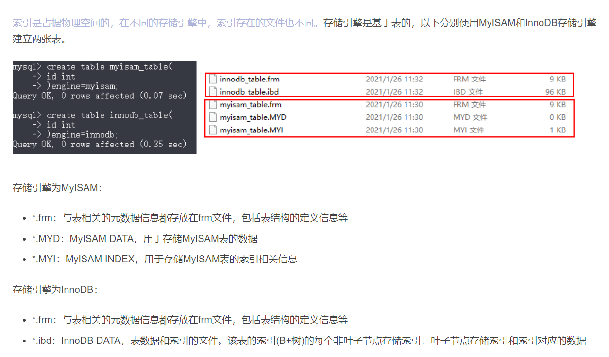
- MySQL index
- 2837xd code generation module learning (4) -- idle_ task、Simulink Coder
- 【JetBrain Rider】构建项目出现异常:未找到导入的项目“D:\VisualStudio2017\IDE\MSBuild\15.0\Bin\Roslyn\Microsoft.CSh
- ERROR 1118 (42000): Row size too large (> 8126)
- Skywalking theory and Practice
- Project practice, redis cluster technology learning (VII)
猜你喜欢


随机推荐
【教程】如何让VisualStudio的HelpViewer帮助文档独立运行
UE5——AI追逐(蓝图、行为树)
Ue5 - ai Pursuit (Blueprint, Behavior tree)
Bookmark collection management software suspension reading and data migration between knowledge base and browser bookmarks
Spatial interpretation | comprehensive analysis of spatial structure of primary liver cancer
[ue5] two implementation methods of AI random roaming blueprint (role blueprint and behavior tree)
2837xd code generation - Supplement (3)
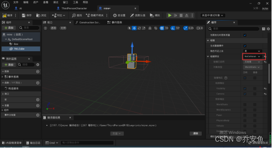
Blender模型导入ue、碰撞设置
Alibaba cloud Prometheus monitoring service
Translation d30 (with AC code POJ 28:sum number)
Junit5 supports suite methods
XA Transaction SQL Statements
What is the relationship between realizing page watermarking and mutationobserver?
[200 Shengxin literatures] 95 multiomics exploration TNBC
【虚幻】过场动画笔记
2837xd code generation module learning (4) -- idle_ task、Simulink Coder
Blender多镜头(多机位)切换
Summary of demand R & D process nodes and key outputs
ERROR 1118 (42000): Row size too large (> 8126)
[leetcode] sword finger offer 53 - I. find the number I in the sorted array