当前位置:网站首页>自然语言处理系列(一)——RNN基础
自然语言处理系列(一)——RNN基础
2022-07-02 09:42:00 【raelum】
注: 本文是总结性文章,叙述较为简洁,不适合初学者
一、为什么要有RNN?
普通的MLP无法处理序列信息(如文本、语音等),这是因为序列是不定长的,而MLP的输入层神经元个数是固定的。
二、RNN的结构
普通MLP的结构(以单隐层为例):
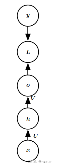
普通RNN(又称Vanilla RNN,接下来都将使用这一说法)的结构(在单隐层MLP的基础上进行改造):

即 t t t 时刻隐藏层接收的输入来自于 t − 1 t-1 t−1 时刻隐藏层的输出和 t t t 时刻的样例输入。用数学公式表示,就是
h ( t ) = tanh ( W h ( t − 1 ) + U x ( t ) + b ) , o ( t ) = V h ( t ) + c , y ^ ( t ) = softmax ( o ( t ) ) h^{(t)}=\tanh(Wh^{(t-1)}+Ux^{(t)}+b),\quad o^{(t)}=Vh^{(t)}+c,\quad \hat{y}^{(t)}=\text{softmax}(o^{(t)}) h(t)=tanh(Wh(t−1)+Ux(t)+b),o(t)=Vh(t)+c,y^(t)=softmax(o(t))
训练RNN的过程中,实际上就是在学习 U , V , W , b , c U,V,W,b,c U,V,W,b,c 这些参数。
正向传播后,我们需要计算损失,设时间步 t t t 处求得的损失为 L ( t ) = L ( t ) ( y ^ ( t ) , y ( t ) ) L^{(t)}=L^{(t)}(\hat{y}^{(t)},y^{(t)}) L(t)=L(t)(y^(t),y(t)),则总的损失为 L = ∑ t = 1 T L ( t ) L=\sum_{t=1}^T L^{(t)} L=∑t=1TL(t)。
2.1 BPTT
BPTT(BackPropagation Through Time),通过时间反向传播是RNN训练过程中的一个术语。因为正向传播时是沿着时间流逝的方向进行的,而反向传播则是逆着时间进行的。
为方便后续推导,我们先改进一下符号表述:
h ( t ) = tanh ( W h h h ( t − 1 ) + W x h x ( t ) + b ) , o ( t ) = W h o h ( t ) + c , y ^ ( t ) = softmax ( o ( t ) ) h^{(t)}=\tanh(W_{hh}h^{(t-1)}+W_{xh}x^{(t)}+b),\quad o^{(t)}=W_{ho}h^{(t)}+c,\quad \hat{y}^{(t)}=\text{softmax}(o^{(t)}) h(t)=tanh(Whhh(t−1)+Wxhx(t)+b),o(t)=Whoh(t)+c,y^(t)=softmax(o(t))
做一个水平方向的 concatenation: W = ( W h h , W x h ) W=(W_{hh},W_{xh}) W=(Whh,Wxh),为简便起见,省略偏置 b b b,则有
h ( t ) = tanh ( W ( h ( t − 1 ) x ( t ) ) ) h^{(t)}=\tanh\left(W \begin{pmatrix} h^{(t-1)} \\ x^{(t)} \end{pmatrix} \right) h(t)=tanh(W(h(t−1)x(t)))
,接下来我们将关注参数 W W W 的学习。
注意到
∂ h ( t ) ∂ h ( t − 1 ) = tanh ′ ( W h h h ( t − 1 ) + W x h x ( t ) ) W h h , ∂ L ∂ W = ∑ t = 1 T ∂ L ( t ) ∂ W \frac{\partial h^{(t)}}{\partial h^{(t-1)}}=\tanh'(W_{hh}h^{(t-1)}+W_{xh}x^{(t)})W_{hh},\quad \frac{\partial L}{\partial W}=\sum_{t=1}^T\frac{\partial L^{(t)}}{\partial W} ∂h(t−1)∂h(t)=tanh′(Whhh(t−1)+Wxhx(t))Whh,∂W∂L=t=1∑T∂W∂L(t)
从而
∂ L ( T ) ∂ W = ∂ L ( T ) ∂ h ( T ) ⋅ ∂ h ( T ) ∂ h ( T − 1 ) ⋯ ∂ h ( 2 ) ∂ h ( 1 ) ⋅ ∂ h ( 1 ) ∂ W = ∂ L ( T ) ∂ h ( T ) ⋅ ∏ t = 2 T ∂ h ( t ) ∂ h ( t − 1 ) ⋅ ∂ h ( 1 ) ∂ W = ∂ L ( T ) ∂ h ( T ) ⋅ ( ∏ t = 2 T tanh ′ ( W h h h ( t − 1 ) + W x h x ( t ) ) ) ⋅ W h h T − 1 ⋅ ∂ h ( 1 ) ∂ W \begin{aligned} \frac{\partial L^{(T)}}{\partial W}&=\frac{\partial L^{(T)}}{\partial h^{(T)}}\cdot \frac{\partial h^{(T)}}{\partial h^{(T-1)}}\cdots \frac{\partial h^{(2)}}{\partial h^{(1)}}\cdot\frac{\partial h^{(1)}}{\partial W} \\ &=\frac{\partial L^{(T)}}{\partial h^{(T)}}\cdot \prod_{t=2}^T\frac{\partial h^{(t)}}{\partial h^{(t-1)}}\cdot\frac{\partial h^{(1)}}{\partial W}\\ &=\frac{\partial L^{(T)}}{\partial h^{(T)}}\cdot \left(\prod_{t=2}^T\tanh'(W_{hh}h^{(t-1)}+W_{xh}x^{(t)})\right)\cdot W_{hh}^{T-1} \cdot\frac{\partial h^{(1)}}{\partial W}\\ \end{aligned} ∂W∂L(T)=∂h(T)∂L(T)⋅∂h(T−1)∂h(T)⋯∂h(1)∂h(2)⋅∂W∂h(1)=∂h(T)∂L(T)⋅t=2∏T∂h(t−1)∂h(t)⋅∂W∂h(1)=∂h(T)∂L(T)⋅(t=2∏Ttanh′(Whhh(t−1)+Wxhx(t)))⋅WhhT−1⋅∂W∂h(1)
因为 tanh ′ ( ⋅ ) \tanh'(\cdot) tanh′(⋅) 几乎总是小于 1 1 1 的,当 T T T 足够大时将会出现梯度消失现象。
假如不采用非线性的激活函数,为简便起见,不妨设激活函数为恒等映射 f ( x ) = x f(x)=x f(x)=x,于是有
∂ L ( T ) ∂ W = ∂ L ( T ) ∂ h ( T ) ⋅ W h h T − 1 ⋅ ∂ h ( 1 ) ∂ W \frac{\partial L^{(T)}}{\partial W}=\frac{\partial L^{(T)}}{\partial h^{(T)}}\cdot W_{hh}^{T-1} \cdot\frac{\partial h^{(1)}}{\partial W} ∂W∂L(T)=∂h(T)∂L(T)⋅WhhT−1⋅∂W∂h(1)
- 当 W h h W_{hh} Whh 的最大奇异值大于 1 1 1 时,会出现梯度爆炸。
- 当 W h h W_{hh} Whh 的最大奇异值小于 1 1 1 时,会出现梯度消失。
三、RNN的分类
按照输入和输出的结构可以对RNN进行如下分类:
- 1 vs N(vec2seq):Image Captioning;
- N vs 1(seq2vec):Sentiment Analysis;
- N vs M(seq2seq):Machine Translation;
- N vs N(seq2seq):Sequence Labeling(POS Tagging)

注意 1 vs 1 是传统的MLP。
若按照内部构造进行分类则会得到:
- RNN、Bi-RNN、…
- LSTM、Bi-LSTM、…
- GRU、Bi-GRU、…
四、Vanilla RNN的优缺点
优点:
- 可以处理不定长的序列;
- 计算时会考虑历史信息;
- 权重沿时间方向上是共享的;
- 模型大小不会随着输入大小增加而改变。
缺点:
- 计算效率低;
- 梯度会消失/爆炸(后续将知道,避免梯度爆炸可采用梯度裁剪,避免梯度消失可换用其他的RNN结构,如LSTM);
- 无法处理长序列(即不具备长记忆性);
- 无法利用未来的输入(Bi-RNN可解决)。
五、Bidirectional RNN
许多时候,我们要输出的 y ( t ) y^{(t)} y(t) 可能依赖于整个序列,因此需要使用双向RNN(BRNN)。BRNN结合了时间上从序列起点开始移动的RNN和从序列末尾开始移动的RNN。两个RNN互相独立不共享权重:
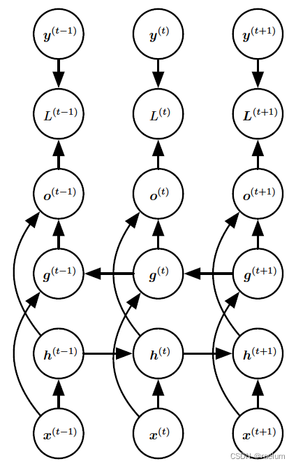
相应的计算方式变为:
h ( t ) = tanh ( W 1 h ( t − 1 ) + U 1 x ( t ) + b 1 ) g ( t ) = tanh ( W 2 h ( t − 1 ) + U 2 x ( t ) + b 2 ) o ( t ) = V ( h ( t ) ; g ( t ) ) + c y ^ ( t ) = softmax ( o ( t ) ) \begin{aligned} &h^{(t)}=\tanh(W_1h^{(t-1)}+U_1x^{(t)}+b_1) \\ &g^{(t)}=\tanh(W_2h^{(t-1)}+U_2x^{(t)}+b_2) \\ &o^{(t)}=V(h^{(t)};g^{(t)})+c \\ &\hat{y}^{(t)}=\text{softmax}(o^{(t)}) \\ \end{aligned} h(t)=tanh(W1h(t−1)+U1x(t)+b1)g(t)=tanh(W2h(t−1)+U2x(t)+b2)o(t)=V(h(t);g(t))+cy^(t)=softmax(o(t))
其中 ( h ( t ) ; g ( t ) ) (h^{(t)};g^{(t)}) (h(t);g(t)) 代表将两个列向量 h ( t ) h^{(t)} h(t) 和 g ( t ) g^{(t)} g(t) 进行纵向连接。
事实上,若将 V V V 按列分块,则上述的第三个等式还可写成:
o ( t ) = V ( h ( t ) ; g ( t ) ) + c = ( V 1 , V 2 ) ( h ( t ) g ( t ) ) + c = V 1 h ( t ) + V 2 g ( t ) + c o^{(t)}=V(h^{(t)};g^{(t)})+c= (V_1,V_2) \begin{pmatrix} h^{(t)} \\ g^{(t)} \end{pmatrix}+c=V_1h^{(t)}+V_2g^{(t)}+c o(t)=V(h(t);g(t))+c=(V1,V2)(h(t)g(t))+c=V1h(t)+V2g(t)+c
训练 BRNN 的过程实际就是在学习 U 1 , U 2 , V , W 1 , W 2 , b 1 , b 2 , c U_1,U_2,V,W_1,W_2,b_1,b_2,c U1,U2,V,W1,W2,b1,b2,c 这些参数。
六、Stacked RNN
堆叠RNN又称多层RNN或深度RNN,即由多个隐藏层组成。以双隐层单向RNN为例,其结构如下:
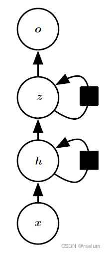
相应的计算过程如下:
h ( t ) = tanh ( W h h h ( t − 1 ) + W x h x ( t ) + b h ) z ( t ) = tanh ( W z z z ( t − 1 ) + W h z h ( t ) + b z ) o ( t ) = W z o z ( t ) + b o y ^ ( t ) = softmax ( o ( t ) ) \begin{aligned} &h^{(t)}=\tanh(W_{hh}h^{(t-1)}+W_{xh}x^{(t)}+b_h) \\ &z^{(t)}=\tanh(W_{zz}z^{(t-1)}+W_{hz}h^{(t)}+b_z) \\ &o^{(t)}=W_{zo}z^{(t)}+b_o \\ &\hat{y}^{(t)}=\text{softmax}(o^{(t)}) \\ \end{aligned} h(t)=tanh(Whhh(t−1)+Wxhx(t)+bh)z(t)=tanh(Wzzz(t−1)+Whzh(t)+bz)o(t)=Wzoz(t)+boy^(t)=softmax(o(t))
边栏推荐
- Pyqt5+opencv project practice: microcirculator pictures, video recording and manual comparison software (with source code)
- Power Spectral Density Estimates Using FFT---MATLAB
- Programmer growth Chapter 6: how to choose a company?
- How to Add P-Values onto Horizontal GGPLOTS
- HOW TO ADD P-VALUES ONTO A GROUPED GGPLOT USING THE GGPUBR R PACKAGE
- HOW TO EASILY CREATE BARPLOTS WITH ERROR BARS IN R
- xss-labs-master靶场环境搭建与1-6关解题思路
- ORB-SLAM2不同线程间的数据共享与传递
- R HISTOGRAM EXAMPLE QUICK REFERENCE
- HOW TO CREATE A BEAUTIFUL INTERACTIVE HEATMAP IN R
猜你喜欢

Seriation in R: How to Optimally Order Objects in a Data Matrice
揭露数据不一致的利器 —— 实时核对系统
YYGH-BUG-04

GGPlot Examples Best Reference

可昇級合約的原理-DelegateCall

HOW TO CREATE A BEAUTIFUL INTERACTIVE HEATMAP IN R
PyTorch搭建LSTM实现服装分类(FashionMNIST)
Research on and off the Oracle chain

Tiktok overseas tiktok: finalizing the final data security agreement with Biden government

Esp32 stores the distribution network information +led displays the distribution network status + press the key to clear the distribution network information (source code attached)
随机推荐
Dynamic debugging of multi file program x32dbg
Log4j2
How to Visualize Missing Data in R using a Heatmap
HOW TO ADD P-VALUES ONTO A GROUPED GGPLOT USING THE GGPUBR R PACKAGE
How to Create a Nice Box and Whisker Plot in R
vant tabs组件选中第一个下划线位置异常
Data analysis - Matplotlib sample code
Enter the top six! Boyun's sales ranking in China's cloud management software market continues to rise
小程序链接生成
The selected cells in Excel form have the selection effect of cross shading
基于 Openzeppelin 的可升级合约解决方案的注意事项
Yygh-9-make an appointment to place an order
A white hole formed by antineutrons produced by particle accelerators
自然语言处理系列(三)——LSTM
QT获取某个日期是第几周
6. Introduce you to LED soft film screen. LED soft film screen size | price | installation | application
Mish-撼动深度学习ReLU激活函数的新继任者
GGHIGHLIGHT: EASY WAY TO HIGHLIGHT A GGPLOT IN R
Precautions for scalable contract solution based on openzeppelin
RPA进阶(二)Uipath应用实践