当前位置:网站首页>自然语言处理系列(三)——LSTM
自然语言处理系列(三)——LSTM
2022-07-02 09:42:00 【raelum】
注: 本文是总结性文章,不适合初学者
一、结构比较
只考虑单隐层单向的RNN,忽略输出层,首先看Vanilla RNN中一个cell的结构:
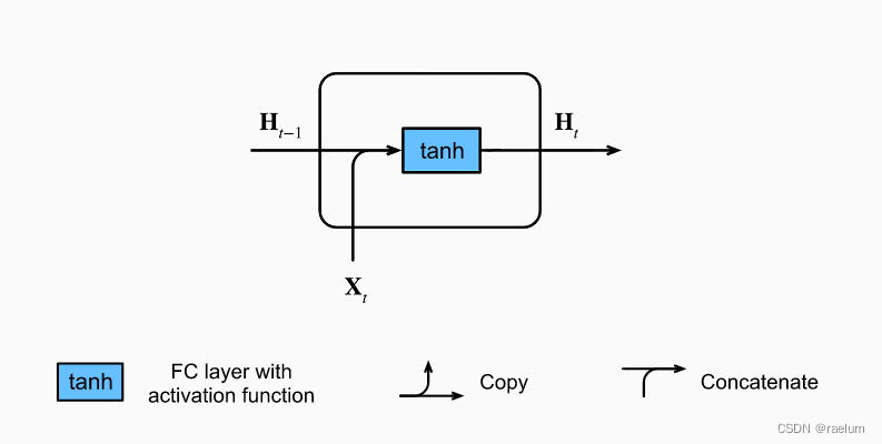
其计算过程为(设批量大小为 N N N,隐层结点个数为 h h h,输入特征数为 d d d):
H t = tanh ( X t W x h + H t − 1 W h h + b h ) {\bf H}_t=\tanh({\bf X}_t{\bf W}_{xh}+{\bf H}_{t-1}{\bf W}_{hh}+{\boldsymbol b}_h) Ht=tanh(XtWxh+Ht−1Whh+bh)
其中各参数的形状为:
- H t , H t − 1 {\bf H}_t,{\bf H}_{t-1} Ht,Ht−1: N × h N\times h N×h;
- X t {\bf X}_t Xt: N × d N\times d N×d;
- W x h {\bf W}_{xh} Wxh: d × h d\times h d×h;
- W h h {\bf W}_{hh} Whh: h × h h\times h h×h;
- b h {\boldsymbol b}_{h} bh: 1 × h 1\times h 1×h。
在计算时, b h {\boldsymbol b}_{h} bh 将利用广播机制从上往下复制成 N × h N\times h N×h 的形状。
LSTM中一个cell的结构:
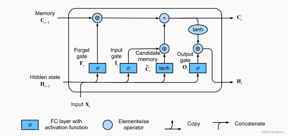
其计算过程为(设 σ ( ⋅ ) \sigma(\cdot) σ(⋅) 代表 Sigmoid ( ⋅ ) \text{Sigmoid}(\cdot) Sigmoid(⋅)):
I t = σ ( X t W x i + H t − 1 W h i + b i ) F t = σ ( X t W x f + H t − 1 W h f + b f ) O t = σ ( X t W x o + H t − 1 W h o + b o ) C ~ t = tanh ( X t W x c + H t − 1 W h c + b c ) C t = F t ⊙ C t − 1 + I t ⊙ C ~ t H t = O t ⊙ tanh ( C t ) \begin{aligned} {\bf I}_t&=\sigma({\bf X}_t{\bf W}_{xi}+{\bf H}_{t-1}{\bf W}_{hi}+{\boldsymbol b}_i) \\ {\bf F}_t&=\sigma({\bf X}_t{\bf W}_{xf}+{\bf H}_{t-1}{\bf W}_{hf}+{\boldsymbol b}_f) \\ {\bf O}_t&=\sigma({\bf X}_t{\bf W}_{xo}+{\bf H}_{t-1}{\bf W}_{ho}+{\boldsymbol b}_o) \\ \tilde{ {\bf C}}_t&=\tanh({\bf X}_t{\bf W}_{xc}+{\bf H}_{t-1}{\bf W}_{hc}+{\boldsymbol b}_c) \\ {\bf C}_t&={\bf F}_t \odot{\bf C}_{t-1}+{\bf I}_t\odot \tilde{ {\bf C}}_t \\ {\bf H}_t&={\bf O}_t\odot \tanh({\bf C}_t) \\ \end{aligned} ItFtOtC~tCtHt=σ(XtWxi+Ht−1Whi+bi)=σ(XtWxf+Ht−1Whf+bf)=σ(XtWxo+Ht−1Who+bo)=tanh(XtWxc+Ht−1Whc+bc)=Ft⊙Ct−1+It⊙C~t=Ot⊙tanh(Ct)
其中 ⊙ \odot ⊙ 是矩阵的 Hadamard 积,各参数的形状如下:
- H t , H t − 1 {\bf H}_t,{\bf H}_{t-1} Ht,Ht−1、 I t , F t , O t {\bf I}_t,{\bf F}_t,{\bf O}_t It,Ft,Ot、 C ~ t , C t , C t − 1 \tilde{ {\bf C}}_t,{\bf C}_t,{\bf C}_{t-1} C~t,Ct,Ct−1: N × h N\times h N×h;
- X t {\bf X}_t Xt: N × d N\times d N×d;
- W x i , W x f , W x o , W x c {\bf W}_{xi},{\bf W}_{xf},{\bf W}_{xo},{\bf W}_{xc} Wxi,Wxf,Wxo,Wxc: d × h d\times h d×h;
- W h i , W h f , W h o , W h c {\bf W}_{hi},{\bf W}_{hf},{\bf W}_{ho},{\bf W}_{hc} Whi,Whf,Who,Whc: h × h h\times h h×h;
- b i , b f , b o , b c {\boldsymbol b}_{i},{\boldsymbol b}_{f},{\boldsymbol b}_{o},{\boldsymbol b}_{c} bi,bf,bo,bc: 1 × h 1\times h 1×h
二、LSTM基础
LSTM一共有三个门: I t , F t , O t {\bf I}_t,{\bf F}_t,{\bf O}_t It,Ft,Ot 分别代表输入门、遗忘门和输出门。输入门用来控制采用多少来自 C ~ t \tilde{ {\bf C}}_t C~t 的新数据,遗忘门用来控制保留多少 C t − 1 {\bf C}_{t-1} Ct−1 的内容,输出门用来控制向下一个时间步传递多少记忆信息。
对于LSTM,只考虑 batch_first=True 的情形,输入数据的形状为 L × N × d L\times N\times d L×N×d。此外还需输入 H 0 {\bf H}_0 H0 和 C 0 {\bf C}_0 C0,其形状均为 1 × N × h 1\times N\times h 1×N×h。
LSTM 在所有时间步上的输出为 [ H 1 , H 2 , ⋯ , H L ] L × N × h [{\bf H}_1,{\bf H}_2,\cdots,{\bf H}_L]_{L\times N\times h} [H1,H2,⋯,HL]L×N×h 和 [ C 1 , C 2 , ⋯ , C L ] L × N × h [{\bf C}_1,{\bf C}_2,\cdots,{\bf C}_L]_{L\times N\times h} [C1,C2,⋯,CL]L×N×h。其中 H t {\bf H}_t Ht 代表 t t t 时刻的隐状态, C t {\bf C}_t Ct 代表 t t t 时刻的记忆。
三、从零开始搭建LSTM
不考虑隐层和输出层之间的参数,可以看出LSTM需要学习的参数一共有 4 4 4 组,即: ( W x ∗ , W h ∗ , b ∗ ) , where ∗ = i , f , o , c ({\bf W}_{x*},{\bf W}_{h*},{\boldsymbol b}_{*}),\; \text{where}\;*=i,f,o,c (Wx∗,Wh∗,b∗),where∗=i,f,o,c。因此我们可以按组去初始化相应的参数。
LSTM需要学习的参数一共有 3 × 4 = 12 3\times4=12 3×4=12 个,相比Vanilla RNN的 3 3 3 个参数多了很多。
首先导入本文代码涉及到的所有包:
import math
import string
import numpy as np
import matplotlib.pyplot as plt

import torch
import torch.nn as nn
import torch.nn.functional as F
我们定义一个函数来初始化一组的参数。注意到每一组参数的形状为 ( d × h , h × h , 1 × h ) (d\times h,h\times h,1\times h) (d×h,h×h,1×h):
def init_group_params(input_size, hidden_size):
    std = math.sqrt(2 / (input_size + hidden_size))
    return nn.Parameter(torch.randn(input_size, hidden_size) * std), \
           nn.Parameter(torch.randn(hidden_size, hidden_size) * std), \
           nn.Parameter(torch.randn(1, hidden_size) * std)
接下来搭建LSTM(模仿 nn.LSTM,即不包含隐层和输出层之间的参数):
class LSTM(nn.Module):

    def __init__(self, input_size, hidden_size):
        super().__init__()
        self.W_xi, self.W_hi, self.b_i = init_group_params(input_size, hidden_size)
        self.W_xf, self.W_hf, self.b_o = init_group_params(input_size, hidden_size)
        self.W_xo, self.W_ho, self.b_f = init_group_params(input_size, hidden_size)
        self.W_xc, self.W_hc, self.b_c = init_group_params(input_size, hidden_size)

    def forward(self, inputs, h_0, c_0):
        L, N, d = inputs.shape
        H, C = h_0[0], c_0[0]
        outputs = []
        for t in range(L):
            X = inputs[t]
            I = torch.sigmoid(X @ self.W_xi + H @ self.W_hi + self.b_i)
            F = torch.sigmoid(X @ self.W_xf + H @ self.W_hf + self.b_f)
            O = torch.sigmoid(X @ self.W_xo + H @ self.W_ho + self.b_o)
            C_temp = torch.tanh(X @ self.W_xc + H @ self.W_hc + self.b_c)
            C = F * C + I * C_temp
            H = O * torch.tanh(C)
            outputs.append(H)
        h_n, c_n = H.unsqueeze(0), C.unsqueeze(0)
        outputs = torch.cat(outputs, 0).unsqueeze(1)
        return outputs, h_n, c_n
最后搭建模型,此时需要加上线性层(输出层):
class Model(nn.Module):

    def __init__(self, input_size, hidden_size, output_size):
        super().__init__()
        self.lstm = LSTM(input_size, hidden_size)
        self.linear = nn.Linear(hidden_size, output_size)

    def forward(self, x):
        # 全零初始化h_0和c_0
        _, h_n, _ = self.lstm(x, torch.zeros(1, x.shape[1], self.linear.in_features).to(device),
                              torch.zeros(1, x.shape[1], self.linear.in_features).to(device))
        return self.linear(h_n[0])
四、测试我们的LSTM
为了验证搭建好的LSTM是正确的模型,我们需要用它来完成一个任务。
4.1 字符预测任务
通俗点来讲,即给定一个单词(长度为 n n n),当模型读取了前 n − 1 n-1 n−1 个字母后,它能够准确地预测出最后一个字母。例如,对于单词 machine,当模型读取完 machin 后,它应当给出预测结果:e。
需要注意的是,字符预测任务并不是完美的。例如给定前两个字母
be,第三个字母无论是e还是t都能构成一个单词,而测试集是有限的,可能只有唯一的答案。
我们使用单词数据集(下载地址),其中训练集包含了 8000 个单词,测试集包含了 2000 个单词,且训练集和测试集没有重合。
4.2 数据预处理
LSTM无法直接识别字母,因此需要先将单个字母转化成张量(one-hot编码):
def letter2tensor(letter):
    letter_idx = torch.tensor(string.ascii_lowercase.index(letter))
    return F.one_hot(letter_idx, num_classes=len(string.ascii_lowercase))
然后再创建一个函数用于将整个单词转化成对应的张量(这里我们将一个单词视为一个 batch,因此形状为 L × 1 × d L\times1\times d L×1×d,其中 d = 26 d=26 d=26, L L L 是单词的长度):
def word2tensor(word):
    result = torch.zeros(len(word), len(string.ascii_lowercase))
    for i in range(len(word)):
        result[i] = letter2tensor(word[i])
    return result.unsqueeze(1)
例如:
print(word2tensor('cat'))
# tensor([[[0., 0., 1., 0., 0., 0., 0., 0., 0., 0., 0., 0., 0., 0., 0., 0., 0.,
# 0., 0., 0., 0., 0., 0., 0., 0., 0.]],

# [[1., 0., 0., 0., 0., 0., 0., 0., 0., 0., 0., 0., 0., 0., 0., 0., 0.,
# 0., 0., 0., 0., 0., 0., 0., 0., 0.]],

# [[0., 0., 0., 0., 0., 0., 0., 0., 0., 0., 0., 0., 0., 0., 0., 0., 0.,
# 0., 0., 1., 0., 0., 0., 0., 0., 0.]]])
读取训练集和测试集:
with open('words/train.txt') as f:
    train_data = f.read().strip().split('\n')

with open('words/test.txt') as f:
    test_data = f.read().strip().split('\n')

print(train_data[0], test_data[1])
# clothe trend
此外,为了保证结果的可复现性,我们还需设置种子:
def setup_seed(seed):
    np.random.seed(seed)
    torch.manual_seed(seed)
    torch.cuda.manual_seed(seed)
    torch.cuda.manual_seed_all(seed)
4.3 训练与测试
我们将在训练集上训练 5 个epoch,因为 batch_size=1,所以每隔 800 个 Iteration 输出一次损失并计算此时模型在测试集上的准确率,最后绘制相应的曲线。
setup_seed(42)

device = 'cuda' if torch.cuda.is_available() else 'cpu'
# 实际上相当于26分类任务,所以输出层神经元个数是26
model = Model(26, 64, 26)
model.to(device)

LR = 7e-3  # 学习率
EPOCHS = 5  # 多少个epoch
INTERVAL = 800  # 多少个iteration输出一次

critertion = nn.CrossEntropyLoss()
# 采用SGD优化器会出现测试集精度不变的情况
optimizer = torch.optim.Adam(model.parameters(), lr=LR, weight_decay=3e-4)

train_loss = []
test_acc = []
avg_train_loss = 0  # 训练集平均损失
correct = 0  # 模型在测试集上预测正确的个数

for epoch in range(EPOCHS):
    print(f'Epoch {
      epoch+1}')
    print('-' * 62)
    for iteration in range(len(train_data)):
        full_word = train_data[iteration]
        # 读取的是前n-1个字母,最后一个字母用作target
        X = word2tensor(full_word[:-1]).to(device)
        target = torch.tensor([string.ascii_lowercase.index(full_word[-1])]).to(device)

        # 正向传播
        output = model(X)
        loss = critertion(output, target)
        avg_train_loss += loss

        # 反向传播
        optimizer.zero_grad()
        loss.backward()
        optimizer.step()

        # 每隔800个iteration输出一次损失并计算模型在测试集上的准确率
        if (iteration + 1) % INTERVAL == 0:
            avg_train_loss /= INTERVAL
            train_loss.append(avg_train_loss.item())

            # 计算模型在测试集上的预测准确率
            with torch.no_grad():
                for test_word in test_data:
                    X = word2tensor(test_word[:-1]).to(device)
                    target = torch.tensor(string.ascii_lowercase.index(test_word[-1])).to(device)
                    pred = model(X)
                    correct += (pred.argmax() == target).sum().item()
                acc = correct / len(test_data)
                test_acc.append(acc)

            print(
                f'Iteration: [{
      iteration + 1:04}/{
      len(train_data)}] | Train Loss: {
      avg_train_loss:.4f} | Test Acc: {
      acc:.4f}'
            )
            avg_train_loss, correct = 0, 0
    print()
这里仅展示最后一个 epoch 的输出:
Epoch 5
--------------------------------------------------------------
Iteration: [0800/8000] | Train Loss: 1.2918 | Test Acc: 0.6000
Iteration: [1600/8000] | Train Loss: 1.1903 | Test Acc: 0.5910
Iteration: [2400/8000] | Train Loss: 1.2615 | Test Acc: 0.6075
Iteration: [3200/8000] | Train Loss: 1.2236 | Test Acc: 0.6015
Iteration: [4000/8000] | Train Loss: 1.2355 | Test Acc: 0.5925
Iteration: [4800/8000] | Train Loss: 1.1314 | Test Acc: 0.6050
Iteration: [5600/8000] | Train Loss: 1.2172 | Test Acc: 0.6045
Iteration: [6400/8000] | Train Loss: 1.1808 | Test Acc: 0.6140
Iteration: [7200/8000] | Train Loss: 1.2092 | Test Acc: 0.6185
Iteration: [8000/8000] | Train Loss: 1.1845 | Test Acc: 0.6040
绘制曲线:
step = INTERVAL / len(train_data)
plt.plot(np.arange(step, EPOCHS + step, step), train_loss, label="train loss")
plt.plot(np.arange(step, EPOCHS + step, step), test_acc, label="test acc")
plt.legend(loc="best", fontsize=12)
plt.xlabel('epoch')
plt.show()
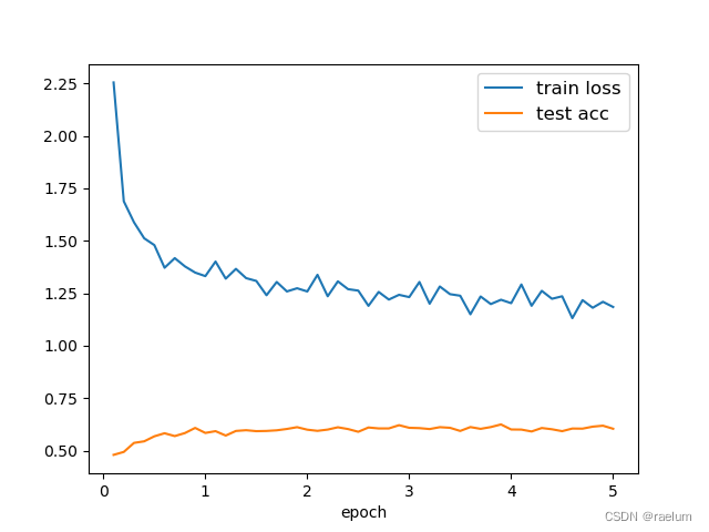
从上图可以看出,模型在测试集上的预测准确率趋于 0.6 0.6 0.6,原因可能有如下几点:
- 数据集的质量不佳;
- 数据集过于简单,LSTM出现了过拟合;
- 我们的任务不够 “自洽”。
边栏推荐
- B high and beautiful code snippet sharing image generation
- GGPUBR: HOW TO ADD ADJUSTED P-VALUES TO A MULTI-PANEL GGPLOT
- Is the stock account given by qiniu business school safe? Can I open an account?
- to_ Bytes and from_ Bytes simple example
- PX4 Position_Control RC_Remoter引入
- QT meter custom control
- QT获取某个日期是第几周
- Is it safe to open a stock account through the QR code of the securities manager? Or is it safe to open an account in a securities company?
- Tdsql | difficult employment? Tencent cloud database micro authentication to help you
- The selected cells in Excel form have the selection effect of cross shading
猜你喜欢

Digital transformation takes the lead to resume production and work, and online and offline full integration rebuilds business logic
Esp32 audio frame esp-adf add key peripheral process code tracking

FLESH-DECT(MedIA 2021)——一个material decomposition的观点

Develop scalable contracts based on hardhat and openzeppelin (I)

Tiktok overseas tiktok: finalizing the final data security agreement with Biden government
YYGH-BUG-04

GGPLOT: HOW TO DISPLAY THE LAST VALUE OF EACH LINE AS LABEL
![[idea] use the plug-in to reverse generate code with one click](/img/b0/00375e61af764a77ea0150bf4f6d9d.png)
[idea] use the plug-in to reverse generate code with one click

PgSQL string is converted to array and associated with other tables, which are displayed in the original order after matching and splicing
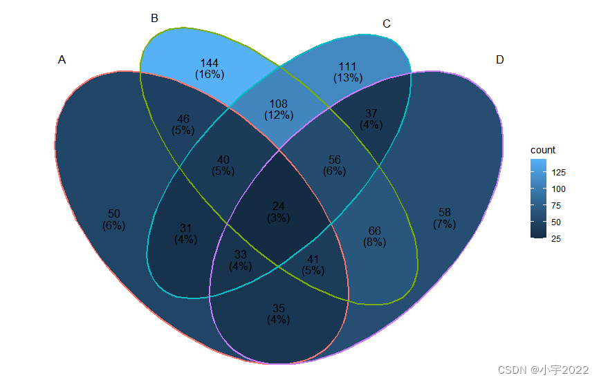
BEAUTIFUL GGPLOT VENN DIAGRAM WITH R
随机推荐
Take you ten days to easily finish the finale of go micro services (distributed transactions)
PHP 2D and multidimensional arrays are out of order, PHP_ PHP scrambles a simple example of a two-dimensional array and a multi-dimensional array. The shuffle function in PHP can only scramble one-dim
基于Hardhat编写合约测试用例
可升级合约的原理-DelegateCall
vant tabs组件选中第一个下划线位置异常
电脑无缘无故黑屏,无法调节亮度。
Log4j2
Always report errors when connecting to MySQL database
GGPlot Examples Best Reference
The selected cells in Excel form have the selection effect of cross shading
R HISTOGRAM EXAMPLE QUICK REFERENCE
How to Add P-Values onto Horizontal GGPLOTS
GGPUBR: HOW TO ADD ADJUSTED P-VALUES TO A MULTI-PANEL GGPLOT
Homer forecast motif
BEAUTIFUL GGPLOT VENN DIAGRAM WITH R
Bedtools tutorial
6. Introduce you to LED soft film screen. LED soft film screen size | price | installation | application
HOW TO EASILY CREATE BARPLOTS WITH ERROR BARS IN R
HOW TO ADD P-VALUES TO GGPLOT FACETS
How to Create a Beautiful Plots in R with Summary Statistics Labels