当前位置:网站首页>Numerical method for solving optimal control problem (0) -- Definition
Numerical method for solving optimal control problem (0) -- Definition
2022-07-07 20:29:00 【Favorite dish of chicken】
Basic description
This article gives a complete description of the optimal control problem .
The optimal control problem can be briefly described as : For a controlled system , Under the constraint conditions , Seek the optimal control quantity to minimize the performance index .
The mathematical description is : Find control variables u ( t ) ∈ R m \boldsymbol{u}(t) \in \mathbb{R}^m u(t)∈Rm, Make the performance index
J = Φ ( x ( t 0 ) , t 0 , x ( t f ) , t f ) + ∫ t 0 t f L ( x ( t ) , u ( t ) , d ) d t J = \Phi (\mathbf{x}(t_0),t_0,\mathbf{x}(t_f),t_f) + \int_{t_0}^{t_f} L(\mathbf{x}(t),\mathbf{u}(t),d) \text{d}t J=Φ(x(t0),t0,x(tf),tf)+∫t0tfL(x(t),u(t),d)dt
Minimum .
The state variables and control variables satisfy the following constraints :
x ˙ ( t ) = f ( x ( t ) , u ( t ) , t ) t ∈ [ t 0 , t f ] , ϕ ( x ( t 0 ) , t 0 , x ( t f ) , t f ) = 0 , C ( x ( t ) , u ( t ) , t ) ≤ 0. \begin{matrix} &\boldsymbol{\dot x}(t) = \boldsymbol{f}(\boldsymbol{x}(t),\boldsymbol{u}(t),t) \quad t \in [t_0,t_f], \\ &\phi (\boldsymbol{x}(t_0),t_0,\boldsymbol{x}(t_f),t_f)=0, \\ &\mathbf{C}(\mathbf{x}(t),\mathbf{u}(t),t) \le 0. \end{matrix} x˙(t)=f(x(t),u(t),t)t∈[t0,tf],ϕ(x(t0),t0,x(tf),tf)=0,C(x(t),u(t),t)≤0.
In style , x ( t ) ∈ R n \boldsymbol{x}(t) \in \mathbb{R}^n x(t)∈Rn Is the state variable , u ( t ) ∈ R m \boldsymbol{u}(t) \in \mathbb{R}^m u(t)∈Rm Is the control variable , t 0 t_0 t0 Is the initial time , t f t_f tf Is the terminal time .
The boundary condition of the state variable satisfies :
x ∈ X ⊂ R n , X = { x ∈ R n : x l o w e r ≤ x ≤ x u p p e r } \boldsymbol{x} \in X \subset \mathbb{R}^n, \quad X = \left \{x \in \mathbb{R}^n: x_{lower} \le x \le x_{upper} \right \} x∈X⊂Rn,X={ x∈Rn:xlower≤x≤xupper}
x l o w e r x_{lower} xlower Is the lower bound of the state variable , x u p p e r x_{upper} xupper Is the upper bound of the state variable .
The boundary condition of the control variable satisfies :
u ∈ U ⊂ R m , U = { u ∈ R m : u l o w e r ≤ u ≤ u u p p e r } \boldsymbol{u} \in U \subset \mathbb{R}^m, \quad U = \left \{u \in \mathbb{R}^m: u_{lower} \le u \le u_{upper} \right \} u∈U⊂Rm,U={ u∈Rm:ulower≤u≤uupper}
u l o w e r u_{lower} ulower Is the lower bound of the control variable , u u p p e r u_{upper} uupper Is the upper bound of the control variable .
Upper form Φ , L , f , ϕ , C \mathit{\Phi}, L, \boldsymbol{f}, \phi, \boldsymbol{C} Φ,L,f,ϕ,C Defined as :
Φ : R n × R × R n × R → R , L : R n × R m × R → R , f : R n × R m × R → R n , ϕ : R n × R × R n × R → R q , f : R n × R m × R → R c , \begin{aligned} &\mathit{\Phi}: \ \mathbb{R}^n \times \mathbb{R} \times \mathbb{R}^n \times \mathbb{R} \rightarrow \mathbb{R}, \\ &L: \ \mathbb{R}^n \times \mathbb{R}^m \times \mathbb{R} \rightarrow \mathbb{R}, \\ &\boldsymbol{f}: \ \mathbb{R}^n \times \mathbb{R}^m \times \mathbb{R} \rightarrow \mathbb{R}^n, \\ &\phi: \ \mathbb{R}^n \times \mathbb{R} \times \mathbb{R}^n \times \mathbb{R} \rightarrow \mathbb{R}^q, \\ &\boldsymbol{f}: \ \mathbb{R}^n \times \mathbb{R}^m \times \mathbb{R} \rightarrow \mathbb{R}^c, \\ \end{aligned} Φ: Rn×R×Rn×R→R,L: Rn×Rm×R→R,f: Rn×Rm×R→Rn,ϕ: Rn×R×Rn×R→Rq,f: Rn×Rm×R→Rc,
Optimal control , The control quantity changes in time sequence , The solution result is several curves . After the control curve is determined , The state curve can be determined according to the differential dynamics system .
Part of the
The above optimal control problem generally consists of four parts , Respectively :
- Performance indicators ;
- Control system differential equation constraints ;
- Boundary constraints ;
- Path Constraint .
Performance indicators
The performance index is the objective function in the optimization problem , However, in the field of optimal control, we call it performance index . Performance index is an important symbol to measure the quality of control system , There are generally three forms , Namely :
- Mayer Type performance index ;
- Lagrange Type performance index ;
- Bolza Type performance index .
Mayer Type performance index
Also known as constant performance index , Only consider the state variables of the control system at the terminal time point 、 Control variables 、 Indicators of time and its composite relationship , Such as the time it takes for the aircraft to move to the specified position ( Terminal time ) etc. . The mathematical description is :
J = Φ ( x ( t 0 ) , t 0 , x ( t f ) , t f ) . J = \Phi (\mathbf{x}(t_0),t_0,\mathbf{x}(t_f),t_f). J=Φ(x(t0),t0,x(tf),tf).
Lagrange Type performance index
Also known as integral performance index , Only emphasize the requirements for the whole control process , This indicator includes the state variables in the whole time domain 、 Integral of control variables and their compound Relations , It can represent the energy consumption of the system , Such as the amount of heat consumption caused by the control process . The mathematical description is :
J = ∫ t 0 t f L ( x ( t ) , u ( t ) , d ) d t . J = \int_{t_0}^{t_f} L(\mathbf{x}(t),\mathbf{u}(t),d) \text{d}t. J=∫t0tfL(x(t),u(t),d)dt.
Bolza Type performance index
Also known as composite performance index , yes Mayer The type and Lagrange Type combination , It not only emphasizes the system state at the time of the terminal , It also emphasizes the requirements for the control system process . This form can be transformed into the above two forms under certain conditions , Therefore, when describing the performance index of general optimal control problems Bolza Type performance index . The mathematical description is :
J = Φ ( x ( t 0 ) , t 0 , x ( t f ) , t f ) + ∫ t 0 t f L ( x ( t ) , u ( t ) , d ) d t . J = \Phi (\mathbf{x}(t_0),t_0,\mathbf{x}(t_f),t_f) + \int_{t_0}^{t_f} L(\mathbf{x}(t),\mathbf{u}(t),d) \text{d}t. J=Φ(x(t0),t0,x(tf),tf)+∫t0tfL(x(t),u(t),d)dt.
Control system differential equation constraints
Optimization problems contain many constraints , The optimal control problem is also a special optimization problem , Its special feature is that the constraint conditions have differential equations .
Any control system needs to use differential equations to describe the motion process , For example, the aircraft is under the action of gravity and thrust , Combined with its own quality changes and other characteristics , Establish a dynamic differential equation that can describe its motion law ; The robot manipulator is subjected to torque , Combine your arm length 、 quality 、 Joint and other characteristics , Establish a dynamic differential equation that can describe its motion law . The above equations can be used as differential algebraic equations (Differential Algebraic Equation,DAE) describe , by :
x ˙ ( t ) = f ( x ( t ) , u ( t ) , t ) t ∈ [ t 0 , t f ] . \boldsymbol{\dot x}(t) = \boldsymbol{f}(\boldsymbol{x}(t),\boldsymbol{u}(t),t) \quad t \in [t_0,t_f]. x˙(t)=f(x(t),u(t),t)t∈[t0,tf].
Boundary constraints
It is often necessary to give the initial state or end state in the control system , Such as the height of the rocket when it was just launched 、 Speed, etc ( The initial state ), You need to specify the height of the rocket at the end 、 Speed, etc ( That is, the end state ). In the optimal control problem , The above state at a certain time point is called boundary constraint . The mathematical description is :
ϕ ( x ( t 0 ) , t 0 , x ( t f ) , t f ) = 0. \phi (\mathbf{x}(t_0),t_0,\mathbf{x}(t_f),t_f) = 0. ϕ(x(t0),t0,x(tf),tf)=0.
Path Constraint
The constraints that the control system must meet in the whole time period are called path constraints .
The difference between path constraints and boundary constraints is , Path constraints occur in the entire time period , Boundary constraints occur at a specific point in time .
Common path constraints include :
- The state variable is on the top of the whole control process 、 Lower limit , Such as aircraft location 、 Speed etc. ;
- The control variable is on the top of the whole control process 、 Lower limit , Such as the output power of the motor 、 Moment, etc ;
- On the function composed of state variables and control variables 、 Lower limit , For example, aircraft or robots need to ensure that they cannot pass through certain specific areas .
The mathematical description of path constraints is :
C ( x ( t ) , u ( t ) , t ) ≤ 0. \mathbf{C}(\mathbf{x}(t),\mathbf{u}(t),t) \le 0. C(x(t),u(t),t)≤0.
summary
thus , So as to give performance indicators 、 Control system differential equation constraints 、 Mathematical description of boundary constraints and path constraints . The above four parts completely define the optimal control problem .
Solve the optimal control problem , That is to solve the optimization problem that minimizes the performance index under the above three kinds of constraints .
边栏推荐
- Splicing and splitting of integer ints
- 最新版本的CodeSonar改进了功能安全性,支持MISRA,C ++解析和可视化
- kubernetes之创建mysql8
- [award publicity] issue 22 publicity of the award list in June 2022: Community star selection | Newcomer Award | blog synchronization | recommendation Award
- 如何满足医疗设备对安全性和保密性的双重需求?
- 恢复持久卷上的备份数据
- CJSON内存泄漏的注意事项
- CodeSonar通过创新型静态分析增强软件可靠性
- Solve the problem of incomplete display around LCD display of rk3128 projector
- 上海交大最新《标签高效深度分割》研究进展综述,全面阐述无监督、粗监督、不完全监督和噪声监督的深度分割方法
猜你喜欢
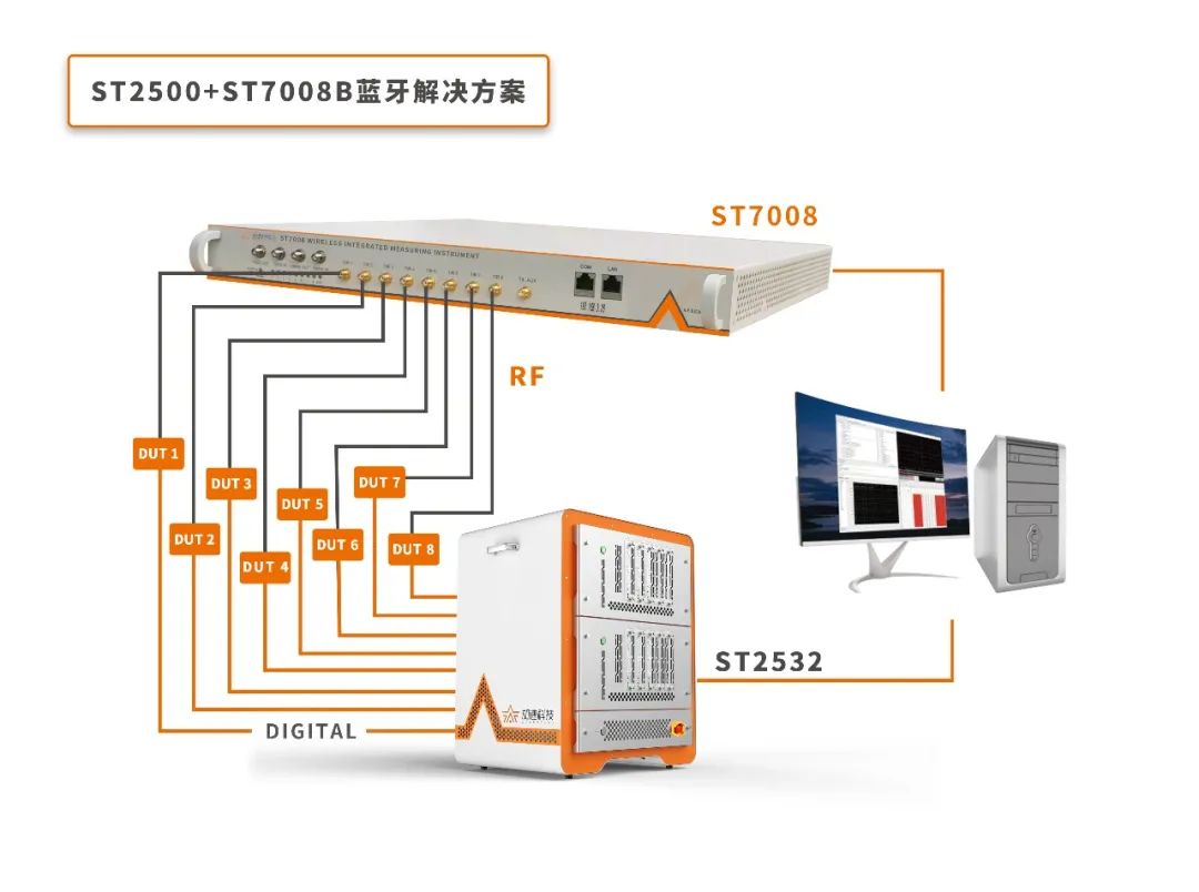
With st7008, the Bluetooth test is completely grasped
Splicing and splitting of integer ints

如何满足医疗设备对安全性和保密性的双重需求?
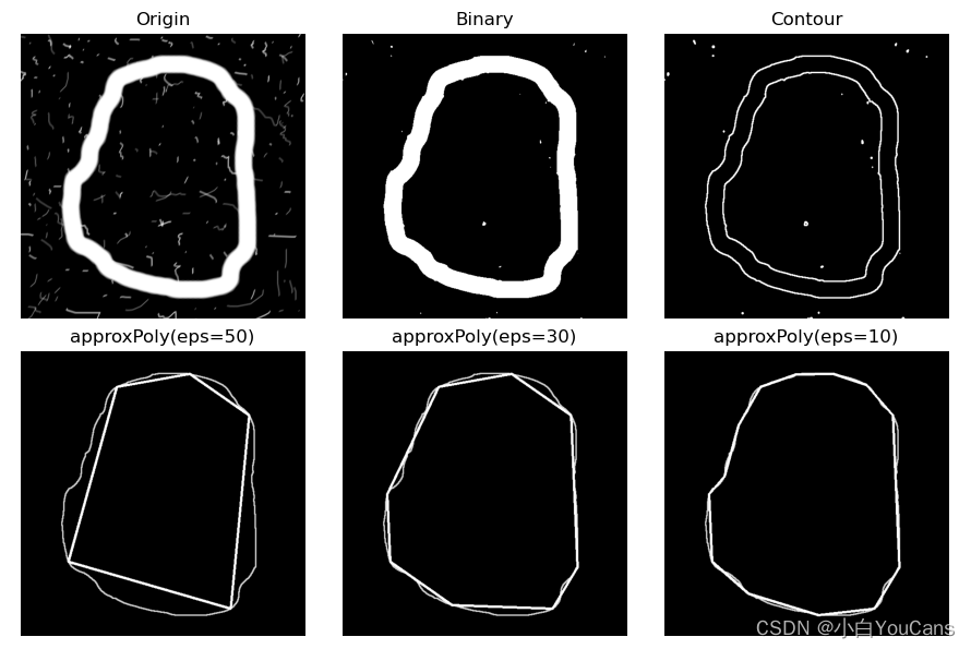
【OpenCV 例程200篇】223. 特征提取之多边形拟合(cv.approxPolyDP)

Machine learning notes - explore object detection datasets using streamlit
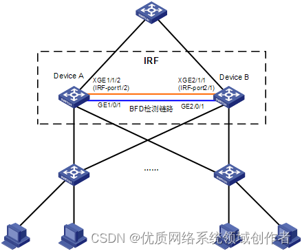
H3C S7000/S7500E/10500系列堆叠后BFD检测配置方法

机械臂速成小指南(十二):逆运动学分析
Micro service remote debug, nocalhost + rainbow micro service development second bullet
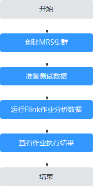
Mrs offline data analysis: process OBS data through Flink job
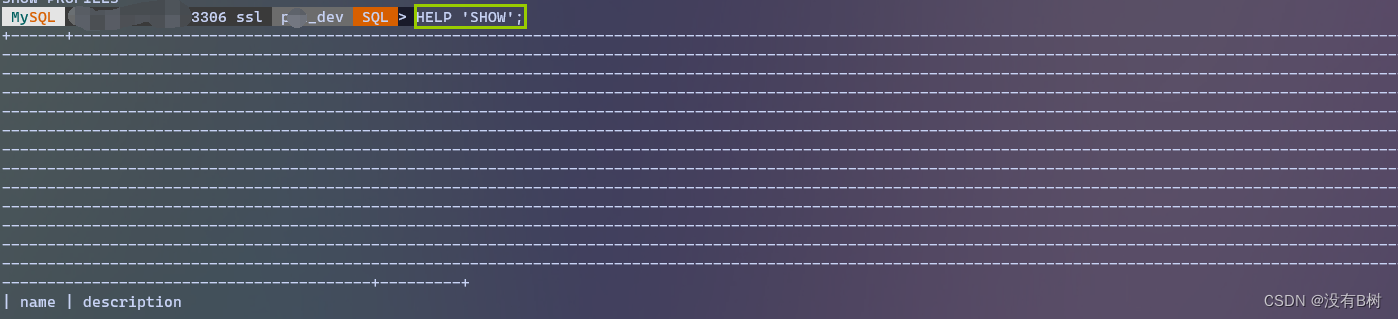
ERROR: 1064 (42000): You have an error in your SQL syntax; check the manual that corresponds to your
随机推荐
如何满足医疗设备对安全性和保密性的双重需求?
Machine learning notes - explore object detection datasets using streamlit
ERROR: 1064 (42000): You have an error in your SQL syntax; check the manual that corresponds to your
I wrote a markdown command line gadget, hoping to improve the efficiency of sending documents by garden friends!
[solution] package 'XXXX' is not in goroot
想杀死某个端口进程,但在服务列表中却找不到,可以之间通过命令行找到这个进程并杀死该进程,减少重启电脑和找到问题根源。
Micro service remote debug, nocalhost + rainbow micro service development second bullet
机械臂速成小指南(十二):逆运动学分析
【函数递归】简单递归的5个经典例子,你都会吗?
凌云出海记 | 赛盒&华为云:共助跨境电商行业可持续发展
Solve the problem that the executable file of /bin/sh container is not found
Measure the height of the building
有用的win11小技巧
[philosophy and practice] the way of program design
目标:不排斥 yaml 语法。争取快速上手
使用高斯Redis实现二级索引
怎样用Google APIs和Google的应用系统进行集成(1)—-Google APIs简介
ISO 26262 - 基于需求测试以外的考虑因素
Small guide for rapid formation of manipulator (12): inverse kinematics analysis
How to implement safety practice in software development stage