当前位置:网站首页>Reprint: defect detection technology of industrial components based on deep learning
Reprint: defect detection technology of industrial components based on deep learning
2022-07-06 18:10:00 【Kamigen】
One 、 Dataset shortcomings
1. The sample size of the dataset is small , There's only... In all 117 A sample picture , There are fewer pictures of defect samples . Insufficient data samples easily lead to the fitting phenomenon of the model , Generalization ability is not strong .
2. The pixel size of the picture is 512*512, Large amount of computation . If the image size is compressed or the image is converted to gray-scale image, it may lead to the loss of useful feature information .
Two 、 Data preprocessing
For the above shortcomings , The simplest and most effective method is to expand the sample size of the data set , Generally, geometric transformation is used to increase the training set samples . The commonly used geometric transformation methods are rotation 、 Zoom translation .
1. Rotation and scaling of pictures
use cv2.getRotationMatrix2D Generating transformation matrix M, Reuse warpAffine Apply affine transformation to the picture . In order to generate multiple pictures with different rotation modes , You can set the rotation angle range , And image zoom range , Take random values in the range every time to generate the rotated picture . The code is as follows ( The code only shows ideas , loosely )
# Set image rotation parameters
RotateOrign=(250,250) # Represents the center of rotation
RotateAngle=(60,90) # It means to rotate clockwise 60-90 degree
RotateScale=(0.8,1) # It means that the image will be scaled to the original after rotation 0.8-1 times

# Define the rotation operation function
def Rotate(image,rotateOrign,rotateAngle,rotateScale):
    img=cv2.imread(image)
    rows,cols=img.shape[:2]
    M=cv2.getRotationMatrix2D(rotateOrign,rotateAngle,rotateScale) # Transformation matrix M
    dst=cv2.warpAffine(img,M,(rows,cols))
    return dst

# Generate pictures
 for item in imgList:
     for num in range(generateImgNum): #generateImgNum: Number of generated pictures
         RotateAngleTmp=random.uniform(RotateAngle[0],RotateAngle[1])
         RotateScaleTmp=random.uniform(RotateScale[0],RotateScale[1])
         outImg=Rotate(item,RotateOrign,RotateAngleTmp,RotateScaleTmp)
         cv2.imwrite(path,outImg)
2. The translation of the picture
First define the translation matrix M, Reuse warpAffine Apply affine transformation to the picture .
# Image translation parameters
MoveX=(50,100) # towards X How many pixel units to move in the direction
MoveY=(-50,50) # towards Y How many pixel units to move in the direction

# Define the translation operation function
def Translate(image,moveX,moveY):
    img=cv2.imread(image)
    M=np.float32([[1,0,moveX],[0,1,moveY]])
    dst=cv2.warpAffine(img,M,img.shape[:2])
    return dst

# Generate pictures
for item in imgList:
    for num in range(generateImgNum): #generateImgNum: Number of generated pictures
        outImg=Translate(item,random.randint(MoveX[0],MoveX[1])
        ,random.randint(MoveY[0],MoveY[1]))
        cv2.imwrite(path,outImg)
In addition to expanding the sample size of the data set through geometric transformation , Common data preprocessing is to extract features from the input image through convolution . Common convolution operations include Gaussian blur and edge detection .
3. Gaussian blur
Gaussian blur , It's also called Gaussian smoothing , It is usually used to reduce image noise and reduce the level of detail ( Baidu Encyclopedia )
use cv2.GaussianBlur Gaussian Blur , The size of Gaussian convolution kernel must be positive and odd .
# Gaussian blur parameter
GaussianBlurkernelSize=5 # The size of Gaussian convolution kernel
GaussianBlurSigma=(0,2) # Gaussian kernel standard deviation range

# Define Gaussian blur function
def GaussianBlur(image,kernelSize,sigma):
    img=cv2.imread(image)
    Gblur=cv2.GaussianBlur(img,(kernelSize,kernelSize),sigma)
    return Gblur

# Blur the picture
for item in imgList:
    for num in range(generateImgNum): #generateImgNum: Number of generated pictures
        GaussianBlurSigmaTmp=random.randint(GaussianBlurSigma[0],GaussianBlurSigma[1])
            outImg=GaussianBlur(item,GaussianBlurkernelSize,GaussianBlurSigmaTmp)
            cv2.imwrite(path,outImg)
4. edge detection
Edge detection extracts the edge features of the picture .Canny Images before and after algorithm processing ( The picture is from OpenCV file ):
Several common algorithms of edge detection :Sobel、Laplacian、Canny.
4.1 Sobel
basis : Up and down the pixel 、 The gray weighted difference between the left and right adjacent points , Reach the extreme value at the edge . First pair x Calculate the gradient of the direction and take the absolute value ( There is less than 0 Pixel value ), Right again y Calculate the gradient of the direction and take the absolute value , Finally, the image is mixed and weighted .
sobelx = cv2.Sobel(img,cv2.CV_64F,1,0,ksize=3) #1,0 Indicates that the calculation direction is x
sobelx = cv2.convertScaleAbs(sobelx) # Take the absolute value

sobely = cv2.Sobel(img,cv2.CV_64F,0,1,ksize=3) #0,1 Indicates that the calculation direction is y
sobely = cv2.convertScaleAbs(sobely) # Take the absolute value

sobelxy = cv2.addWeighted(sobelx, 0.5, sobely, 0.5, 0) # Mixed weighting
4.2 Laplacian
basis : Calculate the second derivative , The value at the maximum change is zero, that is, the edge is zero . Direct use cv2.Laplacian Edge detection .
aplacian = cv2.Laplacian(img, cv2.CV_64F,ksize=3)
laplacian = cv2.convertScaleAbs(laplacian)
4.3 Canny
use cv2.Canny Achieve edge detection .Canny Set high threshold and low threshold in the algorithm , The high threshold distinguishes the object to be extracted from the background , Low threshold is used to smooth the contour .
EdgeDetectionThreshold1=25    # Low threshold
EdgeDetectionThreshold2=250   # High threshold

def EdgeDetection(image,threshold1,threshold2,):
    img=cv2.imread(image)
    edges=cv2.Canny(img,threshold1,threshold2)
    return edges

for item in imgList:
    outImg=EdgeDetection(item,EdgeDetectionThreshold1,EdgeDetectionThreshold2)
    cv2.imwrite(path,outImg)
4.4 Canny Algorithm improvement
reference : An improved adaptive threshold Canny Algorithm
OpenCV Documentation about tradition Canny Introduction of algorithm :Canny Edge Detector
Tradition Canny The realization process of the algorithm :
Image Gaussian filtering . Smooth the image , Eliminate noise .
Calculate the gradient intensity and direction of each pixel in the image .
Apply non maximum suppression . Delete some pixels that are not considered edges , Only candidate edges are preserved .
Apply double threshold detection to determine the edge .
Canny Algorithm improvement :
Use bilateral filtering instead of Gaussian filtering . The kernel function of bilateral filtering is the synthesis result of the kernel of spatial domain and the kernel of pixel domain , At the same time, the spatial domain information and gray similarity are considered , Gaussian filtering only considers the spatial distance between pixels . Bilateral filtering implementation function :cv2.bilateralFilter Realize bilateral filtering ,cv2.adaptiveBilateralFilter Realize adaptive bilateral filtering .
The optimal threshold segmentation method is used to obtain the high threshold , use Otsu Method to determine the low threshold .
————————————————
Copyright notice : This paper is about CSDN Blogger 「 Five six six 」 The original article of , follow CC 4.0 BY-SA Copyright agreement , For reprint, please attach the original source link and this statement .
Link to the original text :https://blog.csdn.net/qq_54000005/article/details/125410538
边栏推荐
- Summary of Android interview questions of Dachang in 2022 (II) (including answers)
- J'aimerais dire quelques mots de plus sur ce problème de communication...
- This article discusses the memory layout of objects in the JVM, as well as the principle and application of memory alignment and compression pointer
- 关于这次通信故障,我想多说几句…
- 虚拟机VirtualBox和Vagrant安装
- 基于STM32+华为云IOT设计的智能路灯
- 历史上的今天:Google 之母出生;同一天诞生的两位图灵奖先驱
- MSF horizontal MSF port forwarding + routing table +socks5+proxychains
- STM32按键状态机2——状态简化与增加长按功能
- adb常用命令
猜你喜欢
![[Android] kotlin code writing standardization document](/img/d5/53d6a75e87af15799bf7e5d6eb92a5.png)
[Android] kotlin code writing standardization document
队列的实现

Pytest learning ----- detailed explanation of the request for interface automation test
Implementation of queue
F200——搭载基于模型设计的国产开源飞控系统无人机
Declval of template in generic programming

There is a gap in traditional home decoration. VR panoramic home decoration allows you to experience the completion effect of your new house

Unity particle special effects series - treasure chest of shining stars
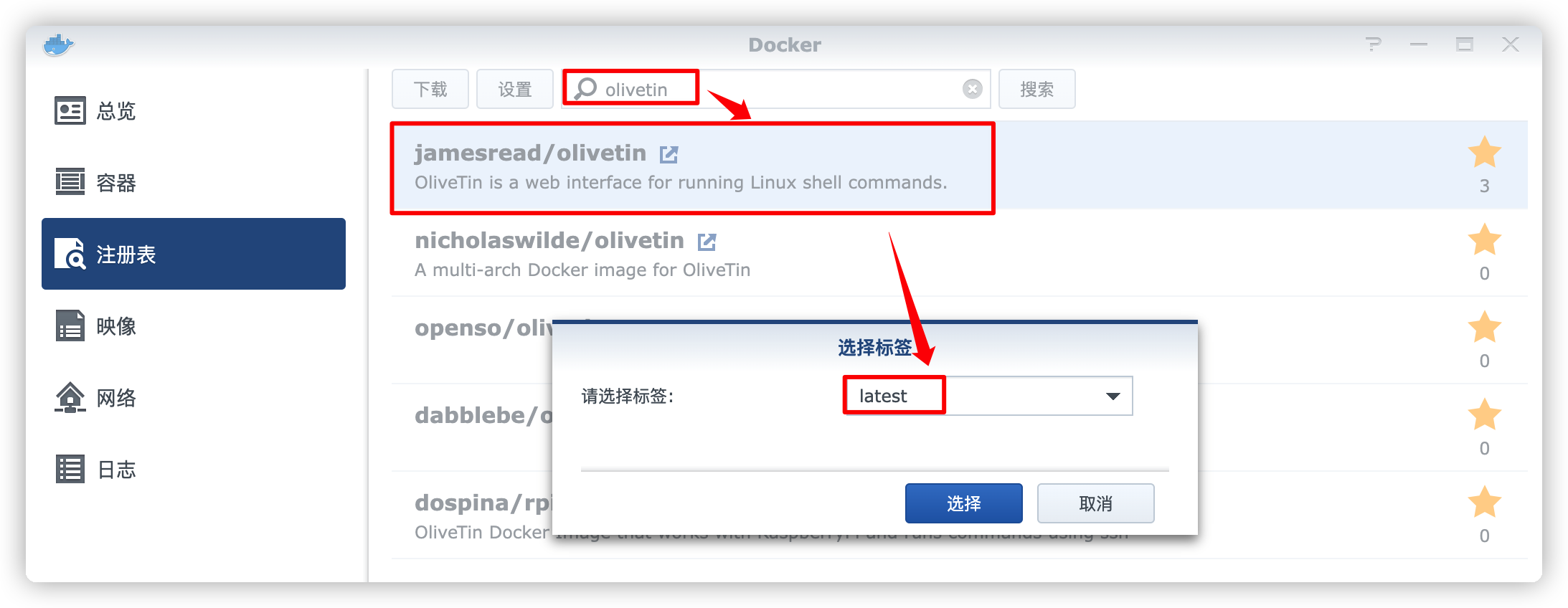
OliveTin能在网页上安全运行shell命令(上)

李书福为何要亲自挂帅造手机?
随机推荐
F200——搭载基于模型设计的国产开源飞控系统无人机
2022暑期项目实训(二)
面试突击63:MySQL 中如何去重?
虚拟机VirtualBox和Vagrant安装
How to solve the error "press any to exit" when deploying multiple easycvr on one server?
二分(整数二分、实数二分)
SAP UI5 框架的 manifest.json
队列的实现
The shell generates JSON arrays and inserts them into the database
Interview shock 62: what are the precautions for group by?
2019 Alibaba cluster dataset Usage Summary
【Swoole系列2.1】先把Swoole跑起来
MS-TCT:Inria&SBU提出用于动作检测的多尺度时间Transformer,效果SOTA!已开源!(CVPR2022)...
ADB common commands
FMT open source self driving instrument | FMT middleware: a high real-time distributed log module Mlog
F200 - UAV equipped with domestic open source flight control system based on Model Design
编译原理——自上而下分析与递归下降分析构造(笔记)
Appium automated test scroll and drag_ and_ Drop slides according to element position
一体化实时 HTAP 数据库 StoneDB,如何替换 MySQL 并实现近百倍性能提升
Will openeuler last long