Natural language processing series (III) -- LSTM

notes ： This article is about Summative article , Not for beginners

One 、 Structure comparison

Only single hidden layer and one-way RNN, Ignore output layer , First of all to see Vanilla RNN In a cell Structure ：

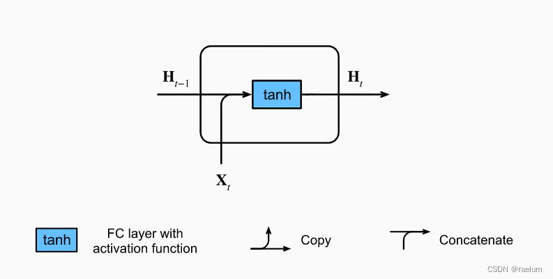
The calculation process is as follows （ Set the batch size to $N$, The number of hidden layer nodes is $h$, The number of input features is $d$）：

$${\mathbf{H}}_t=\tanh ({\mathbf{X}}_t{\mathbf{W}}_{xh}+{\mathbf{H}}_{t-1}{\mathbf{W}}_{hh}+{\mathbf{b}}_h)$$

The shape of each parameter is ：

• ${\mathbf{H}}_t,{\mathbf{H}}_{t-1}$：$N\times h$;
• ${\mathbf{X}}_t$：$N\times d$;
• ${\mathbf{W}}_{xh}$：$d\times h$;
• ${\mathbf{W}}_{hh}$：$h\times h$;
• ${\mathbf{b}}_h$：$1\times h$.

At the time of calculation ,${\mathbf{b}}_h$ The broadcast mechanism will be copied from top to bottom into $N\times h$ The shape of the .

---

LSTM In a cell Structure ：

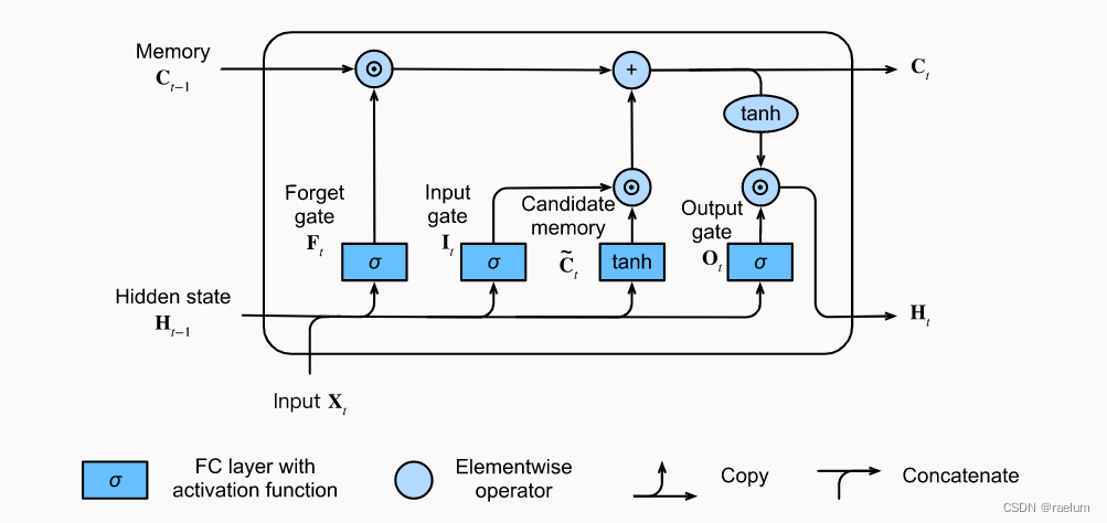
The calculation process is as follows （ set up $\sigma (\cdot )$ representative $\text{Sigmoid}(\cdot )$）：

$$\begin{array}{rl}{\mathbf{I}}_t& =\sigma ({\mathbf{X}}_t{\mathbf{W}}_{xi}+{\mathbf{H}}_{t-1}{\mathbf{W}}_{hi}+{\mathbf{b}}_i)\\ {\mathbf{F}}_t& =\sigma ({\mathbf{X}}_t{\mathbf{W}}_{xf}+{\mathbf{H}}_{t-1}{\mathbf{W}}_{hf}+{\mathbf{b}}_f)\\ {\mathbf{O}}_t& =\sigma ({\mathbf{X}}_t{\mathbf{W}}_{xo}+{\mathbf{H}}_{t-1}{\mathbf{W}}_{ho}+{\mathbf{b}}_o)\\ {\tilde{\mathbf{C}}}_t& =\tanh ({\mathbf{X}}_t{\mathbf{W}}_{xc}+{\mathbf{H}}_{t-1}{\mathbf{W}}_{hc}+{\mathbf{b}}_c)\\ {\mathbf{C}}_t& ={\mathbf{F}}_t\odot {\mathbf{C}}_{t-1}+{\mathbf{I}}_t\odot {\tilde{\mathbf{C}}}_t\\ {\mathbf{H}}_t& ={\mathbf{O}}_t\odot \tanh ({\mathbf{C}}_t)\end{array}$$

among $\odot$ It's matrix Hadamard product , The shape of each parameter is as follows ：

• ${\mathbf{H}}_t,{\mathbf{H}}_{t-1}$、${\mathbf{I}}_t,{\mathbf{F}}_t,{\mathbf{O}}_t$、${\tilde{\mathbf{C}}}_t,{\mathbf{C}}_t,{\mathbf{C}}_{t-1}$：$N\times h$;
• ${\mathbf{X}}_t$：$N\times d$;
• ${\mathbf{W}}_{xi},{\mathbf{W}}_{xf},{\mathbf{W}}_{xo},{\mathbf{W}}_{xc}$：$d\times h$;
• ${\mathbf{W}}_{hi},{\mathbf{W}}_{hf},{\mathbf{W}}_{ho},{\mathbf{W}}_{hc}$：$h\times h$;
• ${\mathbf{b}}_i,{\mathbf{b}}_f,{\mathbf{b}}_o,{\mathbf{b}}_c$：$1\times h$

Two 、LSTM Basics

LSTM There are three doors ：${\mathbf{I}}_t,{\mathbf{F}}_t,{\mathbf{O}}_t$ Each represents the input gate 、 Forgetting gate and output gate . The input gate is used to control how much is used from ${\tilde{\mathbf{C}}}_t$ New data for , Forgetting gate is used to control how much is reserved ${\mathbf{C}}_{t-1}$ The content of , The output gate is used to control how much memory information is transferred to the next time step .

about LSTM, Only consider batch_first=True The circumstances of , The shape of the input data is $L\times N\times d$. In addition, you need to enter ${\mathbf{H}}_0$ and ${\mathbf{C}}_0$, Its shape is $1\times N\times h$.

LSTM The output on all time steps is $[{\mathbf{H}}_1,{\mathbf{H}}_2,\cdots ,{\mathbf{H}}_L{]}_{L\times N\times h}$ and $[{\mathbf{C}}_1,{\mathbf{C}}_2,\cdots ,{\mathbf{C}}_L{]}_{L\times N\times h}$. among ${\mathbf{H}}_t$ representative $t$ The hidden state of time ,${\mathbf{C}}_t$ representative $t$ The memory of the moment .

3、 ... and 、 Build from scratch LSTM

Do not consider the parameters between the hidden layer and the output layer , It can be seen that LSTM There are a total of parameters to learn $4$ Group , namely ：$({\mathbf{W}}_{x\ast },{\mathbf{W}}_{h\ast },{\mathbf{b}}_{\ast }),\text{where}\ast =i,f,o,c$. Therefore, we can initialize the corresponding parameters by groups .

LSTM There are a total of parameters to learn $3\times 4=12$ individual , comparison Vanilla RNN Of $3$ There are many more parameters .

First, import all packages involved in the code in this article ：

import math
import string
import numpy as np
import matplotlib.pyplot as plt

import torch
import torch.nn as nn
import torch.nn.functional as F

We define a function to initialize a set of parameters . Notice that the shape of each set of parameters is $(d\times h,h\times h,1\times h)$：

def init_group_params(input_size, hidden_size):
    std = math.sqrt(2 / (input_size + hidden_size))
    return nn.Parameter(torch.randn(input_size, hidden_size) * std), \
           nn.Parameter(torch.randn(hidden_size, hidden_size) * std), \
           nn.Parameter(torch.randn(1, hidden_size) * std)

Next build LSTM（ imitation nn.LSTM, That is, the parameters between the hidden layer and the output layer are not included ）:

class LSTM(nn.Module):

    def __init__(self, input_size, hidden_size):
        super().__init__()
        self.W_xi, self.W_hi, self.b_i = init_group_params(input_size, hidden_size)
        self.W_xf, self.W_hf, self.b_o = init_group_params(input_size, hidden_size)
        self.W_xo, self.W_ho, self.b_f = init_group_params(input_size, hidden_size)
        self.W_xc, self.W_hc, self.b_c = init_group_params(input_size, hidden_size)

    def forward(self, inputs, h_0, c_0):
        L, N, d = inputs.shape
        H, C = h_0[0], c_0[0]
        outputs = []
        for t in range(L):
            X = inputs[t]
            I = torch.sigmoid(X @ self.W_xi + H @ self.W_hi + self.b_i)
            F = torch.sigmoid(X @ self.W_xf + H @ self.W_hf + self.b_f)
            O = torch.sigmoid(X @ self.W_xo + H @ self.W_ho + self.b_o)
            C_temp = torch.tanh(X @ self.W_xc + H @ self.W_hc + self.b_c)
            C = F * C + I * C_temp
            H = O * torch.tanh(C)
            outputs.append(H)
        h_n, c_n = H.unsqueeze(0), C.unsqueeze(0)
        outputs = torch.cat(outputs, 0).unsqueeze(1)
        return outputs, h_n, c_n

Finally, build the model , At this time, we need to add a linear layer （ Output layer ）：

class Model(nn.Module):

    def __init__(self, input_size, hidden_size, output_size):
        super().__init__()
        self.lstm = LSTM(input_size, hidden_size)
        self.linear = nn.Linear(hidden_size, output_size)

    def forward(self, x):
        #  All zero initialization h_0 and c_0
        _, h_n, _ = self.lstm(x, torch.zeros(1, x.shape[1], self.linear.in_features).to(device),
                              torch.zeros(1, x.shape[1], self.linear.in_features).to(device))
        return self.linear(h_n[0])

Four 、 Test our LSTM

To verify the built LSTM Is the right model , We need it to complete a task .

4.1 Character prediction task

Generally speaking , That is, given a word （ The length is $n$）, When the model is read $n-1$ After two letters , It can accurately predict the last letter . for example , For words machine, When the model is read machin after , It should give a prediction ：e.

It should be noted that , Character prediction tasks are not perfect . For example, given the first two letters be, The third letter is either e still t Can form a word , And the test set is limited , There may be only one answer .

We use word data sets （ Download address ）, The training set contains 8000 Word , The test set contains 2000 Word , And the training set and the test set do not coincide .

4.2 Data preprocessing

LSTM Cannot recognize letters directly , Therefore, we need to convert a single letter into a tensor （one-hot code ）：

def letter2tensor(letter):
    letter_idx = torch.tensor(string.ascii_lowercase.index(letter))
    return F.one_hot(letter_idx, num_classes=len(string.ascii_lowercase))

Then create a function to convert the whole word into the corresponding tensor （ Here we regard a word as a batch, So the shape is $L\times 1\times d$, among $d=26$,$L$ Is the length of the word ）:

def word2tensor(word):
    result = torch.zeros(len(word), len(string.ascii_lowercase))
    for i in range(len(word)):
        result[i] = letter2tensor(word[i])
    return result.unsqueeze(1)

for example ：

print(word2tensor('cat'))
# tensor([[[0., 0., 1., 0., 0., 0., 0., 0., 0., 0., 0., 0., 0., 0., 0., 0., 0.,
# 0., 0., 0., 0., 0., 0., 0., 0., 0.]],

# [[1., 0., 0., 0., 0., 0., 0., 0., 0., 0., 0., 0., 0., 0., 0., 0., 0.,
# 0., 0., 0., 0., 0., 0., 0., 0., 0.]],

# [[0., 0., 0., 0., 0., 0., 0., 0., 0., 0., 0., 0., 0., 0., 0., 0., 0.,
# 0., 0., 1., 0., 0., 0., 0., 0., 0.]]])

Read training set and test set ：

with open('words/train.txt') as f:
    train_data = f.read().strip().split('\n')
    
with open('words/test.txt') as f:
    test_data = f.read().strip().split('\n')
    
print(train_data[0], test_data[1])
# clothe trend

Besides , In order to ensure the reproducibility of the results , We also need to set seeds ：

def setup_seed(seed):
    np.random.seed(seed)
    torch.manual_seed(seed)
    torch.cuda.manual_seed(seed)
    torch.cuda.manual_seed_all(seed)

4.3 Training and testing

We will train on the training set 5 individual epoch, because batch_size=1, So every 800 individual Iteration Output a loss and calculate the accuracy of the model on the test set at this time , Finally, draw the corresponding curve .

setup_seed(42)

device = 'cuda' if torch.cuda.is_available() else 'cpu'
#  In effect 26 Classification task , So the number of neurons in the output layer is 26
model = Model(26, 64, 26)
model.to(device)

LR = 7e-3  #  Learning rate 
EPOCHS = 5  #  How many? epoch
INTERVAL = 800  #  How many? iteration Output a 

critertion = nn.CrossEntropyLoss()
#  use SGD The optimizer will have the same precision of the test set 
optimizer = torch.optim.Adam(model.parameters(), lr=LR, weight_decay=3e-4)

train_loss = []
test_acc = []
avg_train_loss = 0  #  Average loss of training set 
correct = 0  #  The model predicts the correct number on the test set 

for epoch in range(EPOCHS):
    print(f'Epoch {
      epoch+1}')
    print('-' * 62)
    for iteration in range(len(train_data)):
        full_word = train_data[iteration]
        #  Reading is the front n-1 Letters , The last letter is used as target
        X = word2tensor(full_word[:-1]).to(device)
        target = torch.tensor([string.ascii_lowercase.index(full_word[-1])]).to(device)

        #  Positive communication 
        output = model(X)
        loss = critertion(output, target)
        avg_train_loss += loss

        #  Back propagation 
        optimizer.zero_grad()
        loss.backward()
        optimizer.step()

        #  every other 800 individual iteration Output a loss and calculate the accuracy of the model on the test set 
        if (iteration + 1) % INTERVAL == 0:
            avg_train_loss /= INTERVAL
            train_loss.append(avg_train_loss.item())

            #  Calculate the prediction accuracy of the model on the test set 
            with torch.no_grad():
                for test_word in test_data:
                    X = word2tensor(test_word[:-1]).to(device)
                    target = torch.tensor(string.ascii_lowercase.index(test_word[-1])).to(device)
                    pred = model(X)
                    correct += (pred.argmax() == target).sum().item()
                acc = correct / len(test_data)
                test_acc.append(acc)

            print(
                f'Iteration: [{
      iteration + 1:04}/{
      len(train_data)}] | Train Loss: {
      avg_train_loss:.4f} | Test Acc: {
      acc:.4f}'
            )
            avg_train_loss, correct = 0, 0
    print()

Only the last one is shown here epoch Output ：

Epoch 5
--------------------------------------------------------------
Iteration: [0800/8000] | Train Loss: 1.2918 | Test Acc: 0.6000
Iteration: [1600/8000] | Train Loss: 1.1903 | Test Acc: 0.5910
Iteration: [2400/8000] | Train Loss: 1.2615 | Test Acc: 0.6075
Iteration: [3200/8000] | Train Loss: 1.2236 | Test Acc: 0.6015
Iteration: [4000/8000] | Train Loss: 1.2355 | Test Acc: 0.5925
Iteration: [4800/8000] | Train Loss: 1.1314 | Test Acc: 0.6050
Iteration: [5600/8000] | Train Loss: 1.2172 | Test Acc: 0.6045
Iteration: [6400/8000] | Train Loss: 1.1808 | Test Acc: 0.6140
Iteration: [7200/8000] | Train Loss: 1.2092 | Test Acc: 0.6185
Iteration: [8000/8000] | Train Loss: 1.1845 | Test Acc: 0.6040

draw a curve ：

step = INTERVAL / len(train_data)
plt.plot(np.arange(step, EPOCHS + step, step), train_loss, label="train loss")
plt.plot(np.arange(step, EPOCHS + step, step), test_acc, label="test acc")
plt.legend(loc="best", fontsize=12)
plt.xlabel('epoch')
plt.show()

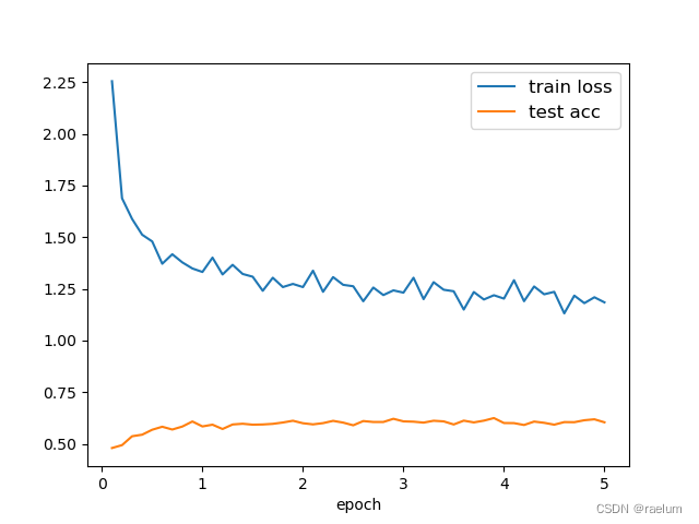
As can be seen from the above figure , The prediction accuracy of the model on the test set tends to $0.6$, The reasons may be as follows ：

• The quality of the dataset is poor ;
• Data sets are too simple ,LSTM There's over fitting ;
• Our task is not enough “ Self consistent ”.