C, Numerical Recipes in C, solution of linear algebraic equations, Gauss Jordan elimination method, source code

 

《Numerical Recipes》 Summary of the original ：

Gauss-Jordan elimination is probably the way you learned to solve linear equa- tions in high school. (You may have learned it as “Gaussian elimination,” but, strictly speaking, that term refers to the somewhat different technique discussed in §2.2.) The basic idea is to add or subtract linear combinations of the given equations until each equation contains only one of the unknowns, thus giving an immediate solution. You might also have learned to use the same technique for calculating the inverse of a matrix.

For solving sets of linear equations, Gauss-Jordan elimination produces both the solution of the equations for one or more right-hand side vectors b, and also the matrix inverse A—1. However, its principal deficiencies are (i) that it requires all the right-hand sides to be stored and manipulated at the same time, and (ii) that when the inverse matrix is not desired, Gauss-Jordan is three times slower than the best alternative technique for solving a single linear set (§2.3). The method’s principal strength is that it is as stable as any other direct method, perhaps even a bit more stable when full pivoting is used (see §2.1.2).

For inverting a matrix, Gauss-Jordan elimination is about as efficient as any other direct method. We know of no reason not to use it in this application if you are sure that the matrix inverse is what you really want.

You might wonder about deficiency (i) above: If we are getting the matrix in- verse anyway, can’t we later let it multiply a new right-hand side to get an additional solution? This does work, but it gives an answer that is very susceptible to roundoff error and not nearly as good as if the new vector had been included with the set of right-hand side vectors in the first instance.

Thus, Gauss-Jordan elimination should not be your method of first choice for solving linear equations. The decomposition methods in §2.3 are better. Why do we discuss Gauss-Jordan at all? Because it is straightforward, solid as a rock, and a good place for us to introduce the important concept of pivoting which will also

be important for the methods described later. The actual sequence of operations performed in Gauss-Jordan elimination is very closely related to that performed by the routines in the next two sections.

Machine translation translation of rounding up words ：

gaussian - Jordan elimination may be the way you learned to solve linear equations in high school .（ You may have understood it as “ Gauss elimination ”, But strictly speaking , The term refers to §2.2 Different technologies discussed in .） The basic idea is to add or subtract linear combinations of given equations , Until each equation contains only one unknown , So as to give the solution immediately . You may also have learned to use the same technique to calculate the inverse of a matrix .

For solving linear equations , gaussian - Jordan elimination generates one or more right-hand vectors b Solution of equation , And matrix inverse A-1. However , Its main defect is （i） It requires that all right sides be stored and operated at the same time , as well as （ii） When inverse matrix is not needed ,Gauss-Jordan Three times slower than the best alternative technique for solving a single linear set （§2.3）. The main advantages of this method are , It is as stable as any other direct method , When using full rotation , Maybe even more stable （ see §2.1.2）.

For matrix inversion , gaussian - Jordan elimination is as effective as any other direct method . If you are sure that the inverse of the matrix is what you really want , Then there's no reason why we don't use it in this application .

You may want to know the defects above （i）： If we get the opposite matrix , Can't we multiply it by a new right-hand side later to get an additional solution ？ It does work , But the answer it gives is easily affected by rounding errors , And it is not as good as the new vector included in the right vector set in the first example .

therefore , gaussian - Jordan elimination method should not be the preferred method for solving linear equations .§2.3 The decomposition method in is better . Why should we talk about Gauss · Jordan ？ Because it is simple and clear , Firm as a rock , It is a good place for us to introduce the important concept of rotation

It is important for the method described later . In Gauss - The actual sequence of operations performed in Jordan elimination is closely related to the sequence of operations performed by the routines in the next two sections .

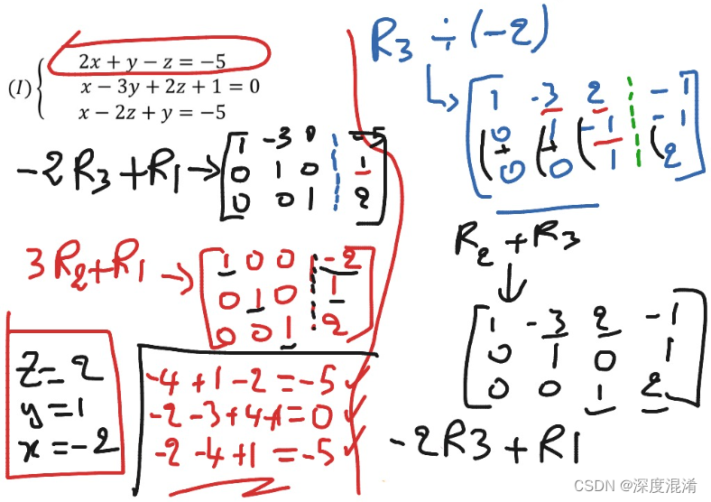
Elimination of column augmentation matrix

For the sake of clarity , And avoid writing endless ellipses （）, We will write only four equations and equations in the case of four unknowns , And it has three different right vectors known in advance . You can write larger matrices , And in a completely similar way, the equation is extended to have M Of the vector on the right side of the Group N The case of a matrix . Of course , Below §2.1.2 The routines implemented in are generic .

 

Select the principal component

In “Gauss-Jordan elimination with no pivoting,” only the second operation in the above list is used. The zeroth row is divided by the element a00 (this being a trivial linear combination of the zeroth row with any other row — zero coefficient for the other row). Then the right amount of the zeroth row is subtracted from each other row to make all the remaining ai0’s zero. The zeroth column of A now agrees with the identity matrix. We move to column 1 and divide row 1 by a11, then subtract the right amount of row 1 from rows 0, 2, and 3, so as to make their entries in column 1 zero. Column 1 is now reduced to the identity form. And so on for columns 2 and 3. As we do these operations to A, we of course also do the corresponding operations to the b’s and to 1 (which by now no longer resembles the identity matrix in any way!). Obviously we will run into trouble if we ever encounter a zero element on the (then current) diagonal when we are going to divide by the diagonal element. (The element that we divide by, incidentally, is called the pivot element or pivot.) Not so obvious, but true, is the fact that Gauss-Jordan elimination with no pivoting (no use of the first or third procedures in the above list) is numerically unstable in the presence of any roundoff error, even when a zero pivot is not encountered. You must never do
Gauss-Jordan elimination (or Gaussian elimination; see below) without pivoting!
So what is this magic pivoting? Nothing more than interchanging rows (partial pivoting) or rows and columns (full pivoting), so as to put a particularly desirable element in the diagonal position from which the pivot is about to be selected. Since we don’t want to mess up the part of the identity matrix that we have already built up, we can choose among elements that are both (i) on rows below (or on) the one that is about to be normalized, and also (ii) on columns to the right (or on) the column we are about to eliminate. Partial pivoting is easier than full pivoting, because we don’t have to keep track of the permutation of the solution vector. Partial pivoting makes available as pivots only the elements already in the correct column. It turns out that partial pivoting is “almost” as good as full pivoting, in a sense that can be made mathematically precise, but which need not concern us here (for discussion and references, see [1]). To show you both variants, we do full pivoting in the routine in this section and partial pivoting in §2.3.
We have to state how to recognize a particularly desirable pivot when we see one. The answer to this is not completely known theoretically. It is known, both theoretically and in practice, that simply picking the largest (in magnitude) available element as the pivot is a very good choice. A curiosity of this procedure, however, is that the choice of pivot will depend on the original scaling of the equations. If we take the third linear equation in our original set and multiply it by a factor of a million, it is almost guaranteed that it will contribute the first pivot; yet the underlying solution

of the equations is not changed by this multiplication! One therefore sometimes sees routines which choose as pivot that element which would have been largest if the original equations had all been scaled to have their largest coefficient normalized to unity. This is called implicit pivoting. There is some extra bookkeeping to keep track of the scale factors by which the rows would have been multiplied. (The routines in
§2.3 include implicit pivoting, but the routine in this section does not.)
Finally, let us consider the storage requirements of the method. With a little reflection you will see that at every stage of the algorithm, either an element of A is predictably a one or zero (if it is already in a part of the matrix that has been reduced to identity form) or else the exactly corresponding element of the matrix that started as 1 is predictably a one or zero (if its mate in A has not been reduced to the identity form). Therefore the matrix 1 does not have to exist as separate storage: The matrix inverse of A is gradually built up in A as the original A is destroyed. Likewise, the solution vectors x can gradually replace the right-hand side vectors b and share the same storage, since after each column in A is reduced, the corresponding row entry in the b’s is never again used.
Here is a routine that does Gauss-Jordan elimination with full pivoting, replac- ing its input matrices by the desired answers. Immediately following is an over- loaded version for use when there are no right-hand sides, i.e., when you want only the matrix inverse.

stay “ Gauss without rotation - Jordan elimination ” in , Use only the second operation in the above list . Line zero divided by element a00（ This is a trivial linear combination of line zero and any other line - The zero coefficient of the other line ）. Then subtract the second line from the other line 0 The correct number of rows , Make all the remaining ai0 zero . Now? ,A Of the 0 The column is consistent with the identity matrix . Let's move to the 1 Column , Will be the first 1 Line divided by a11, And then from the 0、2 and 3 Subtract the appropriate number of 1 That's ok , Make it in the 1 The entry in the column is zero . The first 1 The column is now simplified to the identification form . For the first 2 Column and the first 3 Column , And so on . When we are right A When performing these operations , Of course we are right b and 1 Do the corresponding operation （ up to now , They no longer resemble identity matrices in any way ！）. obviously , When we divide by diagonal elements , If we were （ At that time ） Zero element encountered on diagonal , We will have trouble .（ By the way , The element we divide by is called a pivot element or pivot .） The less obvious but true fact is , In case of any rounding error , Even if zero pivot is not encountered , Gauss without pivot - Jordan elimination （ Do not use the first or third procedure in the above list ） It is numerically unstable . You must not do this

gaussian - Jordan elimination （ Or Gauss elimination ; See below ） No need to rotate ！

So what is this magical rotation ？ Just switch lines （ Partial rotation ） Or rows and columns （ Complete rotation ）, In order to place the specially needed element at the diagonal position of the axis to be selected . Because we don't want to mess up part of the identity matrix we have established , We can choose from the following elements ：（i） Below the line to be normalized （ Or above ）, as well as （ii） On the right column （ Or on the column we are going to eliminate ）. Partial rotation is easier than complete rotation , Because we don't have to track the arrangement of solution vectors . Partial rotation only makes elements that are already in the correct column available as axes . The fact proved that , Partial rotation “ almost ” As good as complete rotation , In a sense , It can be mathematically accurate , But this does not need our attention here （ For discussion and reference , see also [1]）. To show you these two variants , We did a full rotation in the routine in this section , stay §2.3 Part of the rotation is carried out in .

We must explain , When we see a particularly needed axis , How to identify it . The answer to this question is not completely clear in theory . Both in theory and in practice , Simply choose the largest （ Order of magnitude ） Using elements as axes is a very good choice . However , A strange thing about this process is , The choice of axis will depend on the original scale of the equation . If we take the third linear equation in the original set , Multiply it by a factor of onemillion , It is almost guaranteed that it will contribute the first pivot ; However , Potential solutions

This multiplication will not change the equation ！ therefore , People sometimes see routines that choose an element as the axis , If the original equations are scaled , Normalize the maximum coefficient to one , Then this element will be the largest . This is called implicit rotation . There are some extra bookkeeping to track the scale factor multiplied by rows .（ The routine in

§2.3 Including implicit rotation , However, the routines in this section do not include .）

Last , Let's consider the storage requirements of this method . Think about it , You'll find that , At every stage of the algorithm ,a Every element of can be predicted as 1 or 0（ If it is already in a part of the matrix , This part has been simplified into unit form ）, Or from 1 The exact corresponding elements of the starting matrix can be predicted as 1 or 0（ If it's in a The pairing in has not been simplified to the unit form ）. therefore , matrix 1 It does not have to exist as a separate memory ： With primitive A Destruction ,A The inverse of the matrix is A Gradually establish . Again , Solution vector x You can gradually replace the right vector b And share the same storage , Because it is decreasing A After each column in , No longer use b The corresponding line entry in .

Here is a routine , It uses full rotation for Gauss - Jordan Xiaoyuan , Replace its input matrix with the required answer . Followed by an overloaded version , Used when there is no right-hand side , That is, only matrix inverse time is needed .

 

Source program （POWER BY 315SOFT.COM）：

using System;

namespace Legalsoft.Truffer
{
    /// <summary>
    /// Gauss-Jordan decomposition - PTC
    /// Linear equation solution by Gauss-Jordan elimination.
    /// The input matrix is a[0..n - 1][0..n - 1]. b[0..n - 1][0..m - 1] is
    /// input containing the m right-hand side vectors.On output,
    /// a is replaced by its matrix inverse, and b is replaced by
    /// the corresponding set of solution vectors.
    /// </summary>
    public class GaussJordan
    {
        public GaussJordan() { }

        public static void gaussj(double[,] a, double[,] b)
        {
            int n = a.GetLength(0);
            int m = b.GetLength(1);

            // These integer arrays are used for bookkeeping on the pivoting
            int[] indxc = new int[n];
            int[] indxr = new int[n];
            int[] ipiv = new int[n];

            int icol = 0;
            int irow = 0;
            for (int j = 0; j < n; j++)
            {
                ipiv[j] = 0;
            }
            // This is the main loop over the columns to be reduced.
            for (int i = 0; i < n; i++)
            {
                // This is the outer loop of the search for a pivot element.
                double big = 0.0;
                for (int j = 0; j < n; j++)
                {
                    if (ipiv[j] != 1)
                    {
                        for (int k = 0; k < n; k++)
                        {
                            if (ipiv[k] == 0)
                            {
                                if (Math.Abs(a[j, k]) >= big)
                                {
                                    big = Math.Abs(a[j, k]);
                                    irow = j;
                                    icol = k;
                                }
                            }
                        }
                    }
                }
                ++(ipiv[icol]);
                // We now have the pivot element, so we interchange rows, if needed, to put the pivot
                // element on the diagonal.The columns are not physically interchanged, only relabeled:
                // indxc[i], the column of the .i C 1 / th pivot element, is the.i C 1 / th column that is
                // reduced, while indxr[i] is the row in which that pivot element was originally located.
                // If indxr[i] or indxc[i], there is an implied column interchange. With this form of
                // bookkeeping, the solution b's will end up in the correct order, and the inverse matrix
                // will be scrambled by columns.
                if (irow != icol)
                {
                    for (int l = 0; l < n; l++)
                    {
                        Globals.SWAP(ref a[irow, l],ref a[icol, l]);
                    }
                    for (int l = 0; l < m; l++)
                    {
                        Globals.SWAP(ref b[irow, l],ref b[icol, l]);
                    }
                }
                // We are now ready to divide the pivot row by the
                // pivot element, located at irow and icol.
                indxr[i] = irow;
                indxc[i] = icol;
                //if (a[icol, icol] == 0.0)
                if (Math.Abs(a[icol, icol]) <= float.Epsilon)
                {
                    throw new Exception("gaussj: Singular Matrix");
                }
                double pivinv = 1.0 / a[icol, icol];
                a[icol, icol] = 1.0;
                for (int l = 0; l < n; l++)
                {
                    a[icol, l] *= pivinv;
                }
                for (int l = 0; l < m; l++)
                {
                    b[icol, l] *= pivinv;
                }
                // Next, we reduce the rows..., except for the pivot one, of course.
                for (int ll = 0; ll < n; ll++)
                {
                    if (ll != icol)
                    {
                        double dum = a[ll, icol];
                        a[ll, icol] = 0.0;
                        for (int l = 0; l < n; l++)
                        {
                            a[ll, l] -= a[icol, l] * dum;
                        }
                        for (int l = 0; l < m; l++)
                        {
                            b[ll, l] -= b[icol, l] * dum;
                        }
                    }
                }
            }
            for (int l = n - 1; l >= 0; l--)
            {
                if (indxr[l] != indxc[l])
                {
                    for (int k = 0; k < n; k++)
                    {
                        Globals.SWAP(ref a[k, indxr[l]],ref a[k, indxc[l]]);
                    }
                }
            }
        }

        /// <summary>
        /// Overloaded version with no right-hand sides. Replaces a by its inverse.
        /// </summary>
        /// <param name="a"></param>
        public static void gaussj(double[,] a)
        {
            double[,] b = new double[a.GetLength(0), a.GetLength(1)];
            gaussj( a,  b);
        }

    }
}