Skimage learning (3) -- gamma and log contrast adjustment, histogram equalization, coloring gray images

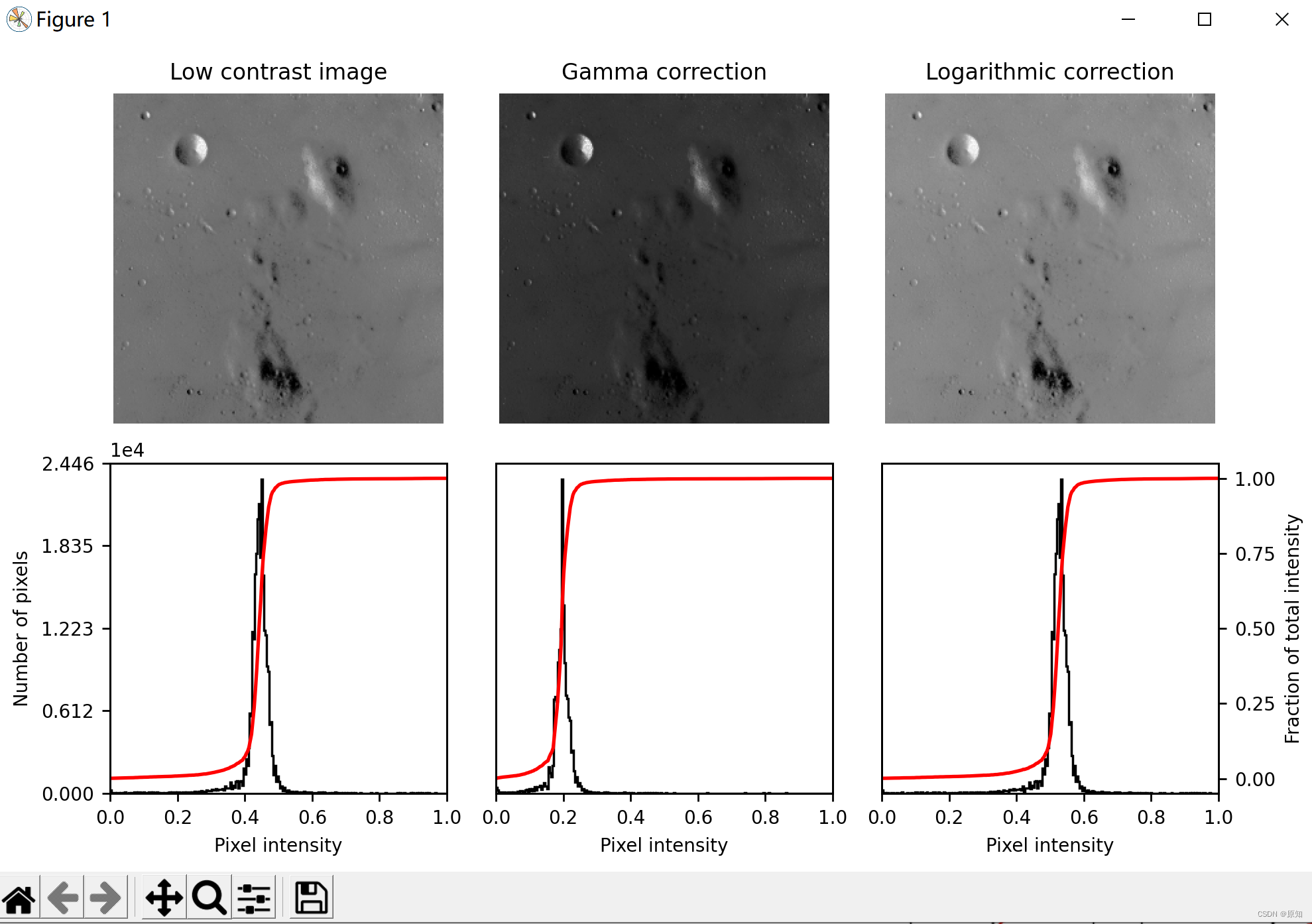
1、Gamma and log Contrast adjustment

This example adjusts the image contrast by performing gamma and logarithmic correction on the input image .

import matplotlib
import matplotlib.pyplot as plt
import numpy as np

from skimage import data, img_as_float
from skimage import exposure

matplotlib.rcParams['font.size'] = 8


def plot_img_and_hist(image, axes, bins=256):
    # Draw the image and its histogram and cumulative histogram .
    image = img_as_float(image)# Convert to floating point 
    ax_img, ax_hist = axes # axes by 2 That's ok 3 Column block , First act ax_img , Second behavior ax_hist
    ax_cdf = ax_hist.twinx() #twinx() The function represents shared x Axis  twiny() It means sharing y Axis   The shared representation is the second row of all coordinate systems x The axis uses the same scale mark 

    # Display image
    ax_img.imshow(image, cmap=plt.cm.gray)
    ax_img.set_axis_off()
    ''' Cmap yes MATLAB The function used to set and obtain the current color map , You can set the following color chart ： hot  Smooth transition from black to red 、 Orange and yellow background colors , Then go to white . cool  Contains shades of turquoise and magenta . From turquoise to magenta . gray  Returns the linear grayscale color map . bone  Grayscale color map with high blue component . This color map is used to add an electronic view to the grayscale map . white  All white monochromatic graph . spring  Contains magenta and yellow shadow colors . summer  Contains green and yellow shadow colors . autumn  Smooth change from red to orange , Then go to yellow . winter  Contains shades of blue and green . '''
    # Display histogram
    ax_hist.hist(image.ravel(), bins=bins, histtype='step', color='black')
    # bins  Is the number of columns in the histogram  image.ravel()  Stretch the matrix into a one-dimensional array 
    # histtype:  Histogram Type ,‘bar’, ‘barstacked’, ‘step’, ‘stepfilled’
    ax_hist.ticklabel_format(axis='y', style='scientific', scilimits=(0, 0))
    #  Set up y Axis 
    # sytle： sci or scientific  Scientific enumeration  plain： Natural number 
    # sclimits (m, n)  The value range of the axis  10 Of m Power  to 10 Of n Power  （0,0） Means unlimited 
    ax_hist.set_xlabel('Pixel intensity')## Set up  x Axis labels ： Pixel strength 
    ax_hist.set_xlim(0, 1)# Set up x Axis range 0 To 1
    ax_hist.set_yticks([])
    # set_xticks  And  set_yticks  Method can be used to set the position of the label 
    # ax.set_xticks([0.25, 0.5, 0.75])
    # ax.set_xticklabels(['a', 'b', 'c'], fontsize=18)

    # Display cumulative distribution
    #  Returns the cumulative distribution function of a given image （cdf） mg_cdf： The value of the array cumulative distribution function .bin_centers： Array center .
    img_cdf, bins = exposure.cumulative_distribution(image, bins)
    ax_cdf.plot(bins, img_cdf, 'r')
    ax_cdf.set_yticks([])

    return ax_img, ax_hist, ax_cdf


# Load an example image
img = data.moon()

# Gamma
gamma_corrected = exposure.adjust_gamma(img, 2)
'''  Adjustment of image brightness and contrast , It's on the skimage Bag exposure Inside the module  gamma adjustment   principle ：I=Ig  For the pixels of the original image , Perform power operation , Get the new pixel value . Formula g Namely gamma value .  If gamma>1,  The new image is darker than the original image   If gamma<1, The new image is brighter than the original image   The function format is ：skimage.exposure.adjust_gamma(image, gamma=1) gamma The parameter defaults to 1, The original image does not change  .  Gamma transform is low for image contrast , And the overall brightness value is high （ For camera overexposure ） In this case, the image enhancement effect is obvious . '''

#  logarithm 
logarithmic_corrected = exposure.adjust_log(img, 1)
''' log  Expression of function : y=alog(1+x), a  Is an amplification factor ,x  It is also the input pixel value , The value range is  [0−1], y  Is the output pixel value .  The logarithmic transformation has a better effect on the image with low overall contrast and low gray value . '''

#  Show results 
fig = plt.figure(figsize=(8, 5))
axes = np.zeros((2, 3), dtype=np.object)#axes The values of two rows and three columns are 0
axes[0, 0] = plt.subplot(2, 3, 1)
axes[0, 1] = plt.subplot(2, 3, 2, sharex=axes[0, 0], sharey=axes[0, 0])
axes[0, 2] = plt.subplot(2, 3, 3, sharex=axes[0, 0], sharey=axes[0, 0])
axes[1, 0] = plt.subplot(2, 3, 4)
axes[1, 1] = plt.subplot(2, 3, 5)
axes[1, 2] = plt.subplot(2, 3, 6)

ax_img, ax_hist, ax_cdf = plot_img_and_hist(img, axes[:, 0])# The first column of the canvas 
ax_img.set_title('Low contrast image')# Low contrast images 

y_min, y_max = ax_hist.get_ylim()
ax_hist.set_ylabel('Number of pixels')# The number of pixels 
ax_hist.set_yticks(np.linspace(0, y_max, 5))#y Axis 5 Equal division , Mark the equal value 

ax_img, ax_hist, ax_cdf = plot_img_and_hist(gamma_corrected, axes[:, 1])
ax_img.set_title('Gamma correction')# Gamma correction 

ax_img, ax_hist, ax_cdf = plot_img_and_hist(logarithmic_corrected, axes[:, 2])
ax_img.set_title('Logarithmic correction')# Logarithmic correction 

ax_cdf.set_ylabel('Fraction of total intensity')# Percentage of total strength 
ax_cdf.set_yticks(np.linspace(0, 1, 5))# Set up y Axis labels 

# prevent overlap of y-axis labels
fig.tight_layout()
plt.show()

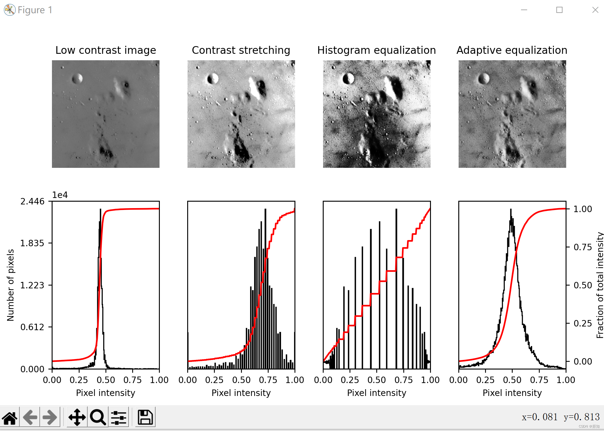
2、 Histogram equalization

This example uses a method called histogram equalization to enhance low contrast images , The method In the image 1 in “ Expand the most frequent intensity value ” . The equalized image has a roughly linear cumulative distribution function .

Although histogram equalization has the advantage of not requiring parameters , But sometimes it will produce images that look unnatural . The other way is Contrast stretch , Where the image is rescaled to include falling on the 2 And the 98 All intensities within the percentile .

import matplotlib
import matplotlib.pyplot as plt
import numpy as np

from skimage import data, img_as_float
from skimage import exposure


matplotlib.rcParams['font.size'] = 8


def plot_img_and_hist(image, axes, bins=256):
    """ Draw the image and its histogram and cumulative histogram . """
    image = img_as_float(image)
    ax_img, ax_hist = axes
    ax_cdf = ax_hist.twinx()

    #  Show pictures 
    ax_img.imshow(image, cmap=plt.cm.gray)
    ax_img.set_axis_off()

    #  Show histogram 
    ax_hist.hist(image.ravel(), bins=bins, histtype='step', color='black')
    ax_hist.ticklabel_format(axis='y', style='scientific', scilimits=(0, 0))
    ax_hist.set_xlabel('Pixel intensity')
    ax_hist.set_xlim(0, 1)
    ax_hist.set_yticks([])

    #  Show cumulative distribution 
    img_cdf, bins = exposure.cumulative_distribution(image, bins)
    ax_cdf.plot(bins, img_cdf, 'r')
    ax_cdf.set_yticks([])

    return ax_img, ax_hist, ax_cdf


#  Load a sample image 
img = data.moon()

#  Contrast stretch , Contrast stretching is a method of image enhancement , It also belongs to grayscale transformation operation 
p2, p98 = np.percentile(img, (2, 98))# What to calculate （2,98） Number sequence . Calculates the second of the data along the specified axis q One hundredth 
img_rescale = exposure.rescale_intensity(img, in_range=(p2, p98))# The original pixel value does not want to be stretched , Just wait for the scale to shrink 
''' numpy.percentile:https://www.cjavapy.com/article/1087/ exposure.rescale_intensity:https://blog.csdn.net/PresleyR/article/details/116200390 '''

#  equilibrium 
img_eq = exposure.equalize_hist(img)

#  Adaptive equalization 
img_adapteq = exposure.equalize_adapthist(img, clip_limit=0.03)

#  Show results 
fig = plt.figure(figsize=(8, 5))
axes = np.zeros((2, 4), dtype=np.object)
axes[0, 0] = fig.add_subplot(2, 4, 1)
for i in range(1, 4):
    axes[0, i] = fig.add_subplot(2, 4, 1+i, sharex=axes[0,0], sharey=axes[0,0])
for i in range(0, 4):
    axes[1, i] = fig.add_subplot(2, 4, 5+i)

ax_img, ax_hist, ax_cdf = plot_img_and_hist(img, axes[:, 0])
ax_img.set_title('Low contrast image')

y_min, y_max = ax_hist.get_ylim()
ax_hist.set_ylabel('Number of pixels')
ax_hist.set_yticks(np.linspace(0, y_max, 5))

ax_img, ax_hist, ax_cdf = plot_img_and_hist(img_rescale, axes[:, 1])
ax_img.set_title('Contrast stretching')# Contrast stretch 

ax_img, ax_hist, ax_cdf = plot_img_and_hist(img_eq, axes[:, 2])
ax_img.set_title('Histogram equalization')# Histogram equalization 

ax_img, ax_hist, ax_cdf = plot_img_and_hist(img_adapteq, axes[:, 3])
ax_img.set_title('Adaptive equalization')# Adaptive equalization 

ax_cdf.set_ylabel('Fraction of total intensity')# Fraction of total intensity 
ax_cdf.set_yticks(np.linspace(0, 1, 5))

#  prevent y Axis labels overlap 
fig.tight_layout()
plt.show()

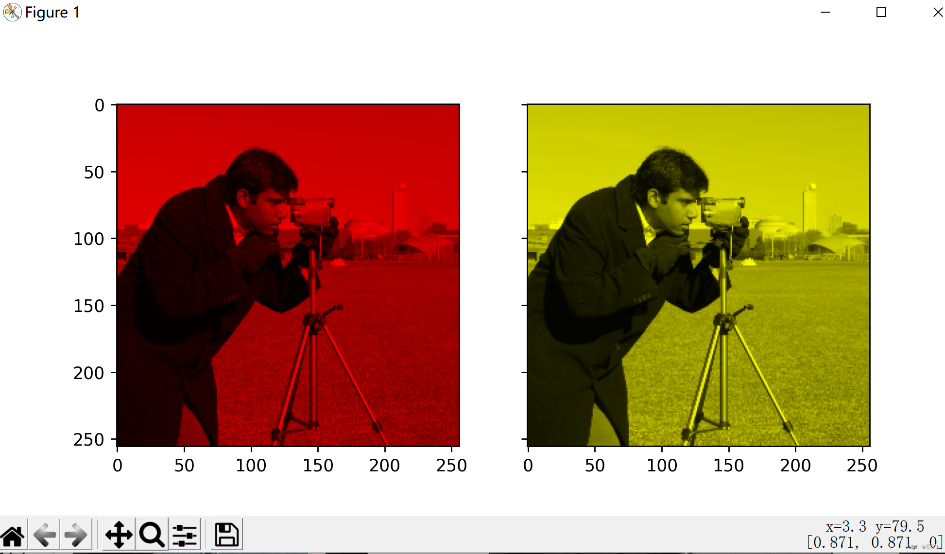
3、 Color grayscale images

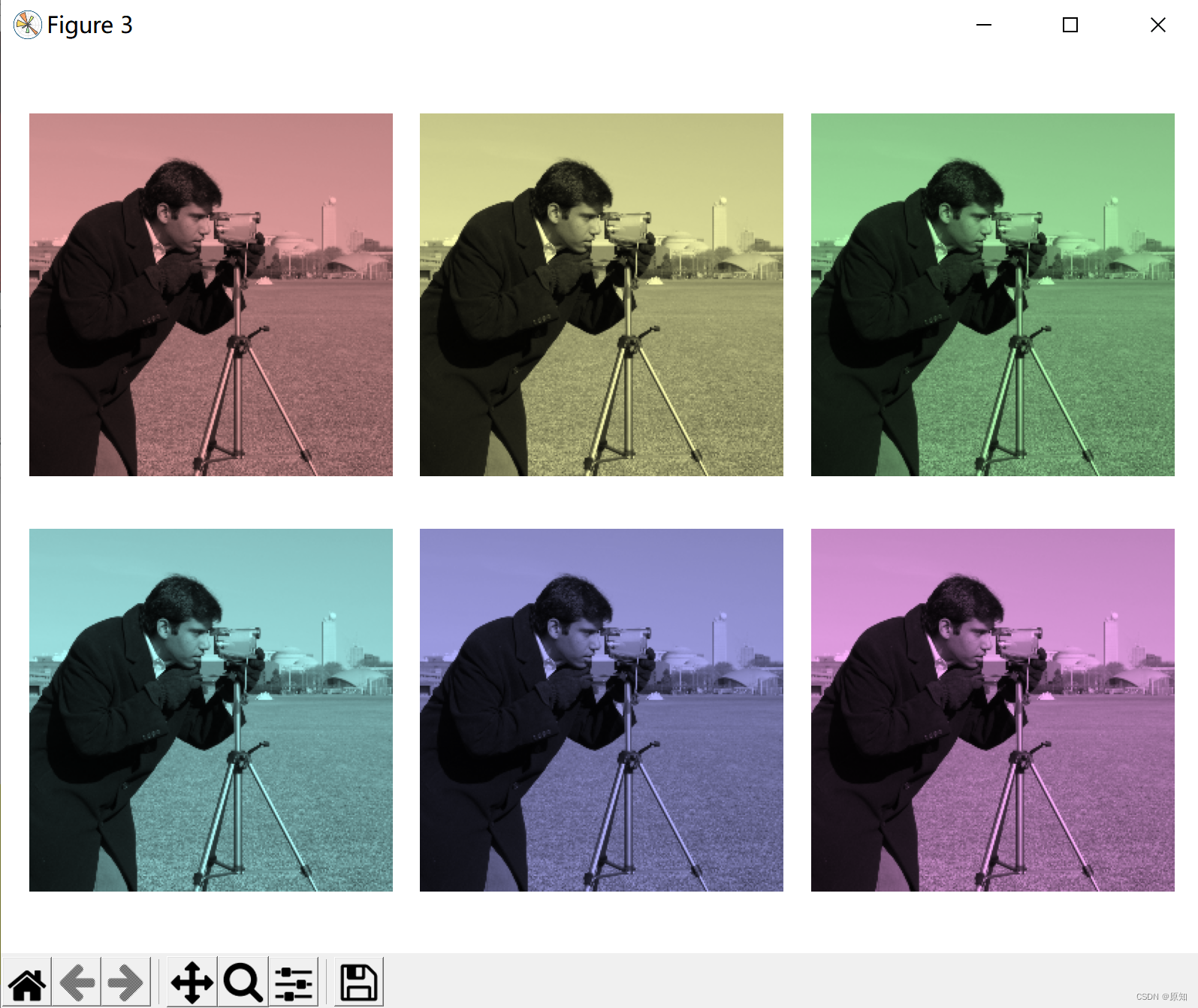
It is very useful to artificially color an image with a certain color , It can highlight specific areas of the image , It can also make grayscale images vivid .
This example is scaled RGB Value and in HSV Adjust colors in color space to demonstrate image shading .
stay 2D in , Color images are usually used 2D Array of RGB-3 The layer said , this 3 Layers represent the ed、(G) green and (B)lue passageway .
The easiest way to get a shaded image is to put each RGB Channels are set to grayscale images scaled by different multipliers for each channel .

'''  for example , Multiply the green and blue channels by 0 Only red channels will be left and bright red images will be produced .  Again , Zero the blue channel , Only red and green channels are left , They combine to form a yellow channel . '''
import matplotlib.pyplot as plt
from skimage import data
from skimage import color
from skimage import img_as_float

grayscale_image = img_as_float(data.camera()[::2, ::2])# Floating point grayscale 
image = color.gray2rgb(grayscale_image)# Create a grayscale image RGB Express .

red_multiplier = [1, 0, 0]
yellow_multiplier = [1, 1, 0]

fig, (ax1, ax2) = plt.subplots(ncols=2, figsize=(8, 4),
                               sharex=True, sharey=True)
ax1.imshow(red_multiplier * image)# Multiply the green and blue channels by 0 Only red channels will be left and bright red images will be produced 
ax2.imshow(yellow_multiplier * image)# Zero the blue channel , Only red and green channels are left , They combine to form a yellow channel 

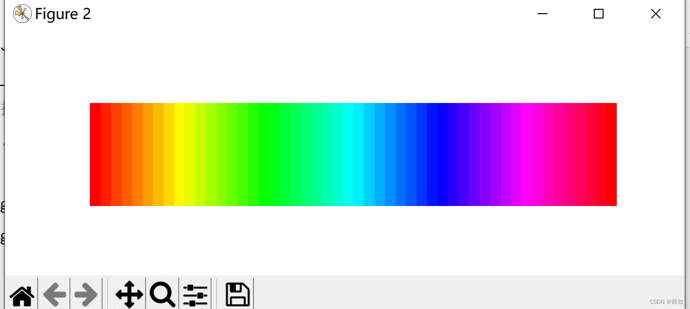
'''  in many instances , Handle RGB The value may not be ideal . Because of that , There are many other color spaces that can be used to represent color images .  A popular color space is called HSV, It represents hue (~ Color )、 saturation (~ Chromaticity ) And the value (~ brightness ).  for example , A color ( tonal ) It may be green , But its saturation is green intensity —— Olive is at the low end , Neon lights are at the high end .  In some implementations ,HSV The hue in the is from 0 To 360, Because the hue is surrounded by a circle .  However , stay scikit-image in , The hue is from 0 To 1 Floating value of , So tone 、 Saturation and value share the same scale .  below , We draw a linear gradient in the hue , Saturation and value rise all the way : '''
import numpy as np

hue_gradient = np.linspace(0, 1)# Again 0、1 The generation length between is 50 Array of 
hsv = np.ones(shape=(1, len(hue_gradient), 3), dtype=float)# Return length is 1, Wide for 50, High for 3 Array of 
hsv[:, :, 0] = hue_gradient

all_hues = color.hsv2rgb(hsv)# Create a grayscale image RGB Express 

fig, ax = plt.subplots(figsize=(5, 2))
#  Set the image range , Change the hue from 0 To 1, Image is a good aspect ratio .
ax.imshow(all_hues, extent=(0 - 0.5 / len(hue_gradient),
                            1 + 0.5 / len(hue_gradient), 0, 0.2))
ax.set_axis_off()

'''  Create a small utility function to get  RGB  Images , also ： 1.  take  RGB  Image to  HSV 2.  Set hue and saturation  3.  take  HSV  Image conversion back to  RGB '''
def colorize(image, hue, saturation=1):
    """  Add the color of the given hue to RGB Image .  By default , Saturation is set to 1, So that the color pops up ! """
    hsv = color.rgb2hsv(image)
    hsv[:, :, 1] = saturation# saturation （S）
    hsv[:, :, 0] = hue# tonal （H）
    return color.hsv2rgb(hsv)

'''  Please note that , We need to increase saturation ; Images with zero saturation are grayscale , So we need a non-zero value to really see the color we set .  Use the function above , We drew six images with linear gradient hue and non-zero saturation ： '''
hue_rotations = np.linspace(0, 1, 7)# Return length is 6, stay 0、1 An array evenly divided between 

fig, axes = plt.subplots(nrows=2, ncols=3, sharex=True, sharey=True)

for ax, hue in zip(axes.flat, hue_rotations):
    # Turn down the saturation to give it that vintage look.
    tinted_image = colorize(image, hue, saturation=0.3)# The saturation is 0.3,hue=hue_rotations
    ax.imshow(tinted_image, vmin=0, vmax=1)
    ax.set_axis_off()
fig.tight_layout()

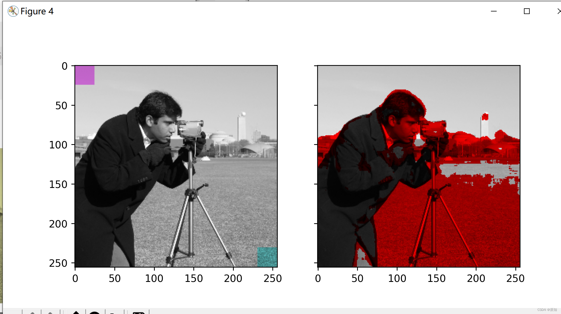
'''  Compare this shading effect with  numpy  Slicing and fine indexing , To selectively color your image .  In the following example , We use slices to set the hue of some rectangles , And scale some pixels found by threshold processing  RGB  value .  In practice , You may want to define a shaded area according to the segmentation result or the speckle detection method . '''
from skimage.filters import rank

#  A square area defined as a slice on the first two dimensions .
top_left = (slice(25),) * 2#slice() Function to implement slicing objects ,x Axis and y Axis 
bottom_right = (slice(-25, None),) * 2
print("top_left:",top_left)
print("bottom_right:",bottom_right)
#top_left: (slice(None, 25, None), slice(None, 25, None))
#bottom_right: (slice(-25, None, None), slice(-25, None, None))
sliced_image = image.copy()
sliced_image[top_left] = colorize(image[top_left], 0.82, saturation=0.5)# Section staining 
sliced_image[bottom_right] = colorize(image[bottom_right], 0.5, saturation=0.5)

#  Create a mask selection area with interesting textures .
noisy = rank.entropy(grayscale_image, np.ones((9, 9)))
''' skimage.filters.rank.entropy(image,footprint,out = None,mask = None,shift_x = False,shift_y = False,shift_z = False）  Entropy is used in  2  Base logarithm calculation , That is, the filter returns the minimum number of bits required to encode the local gray distribution   Parameters ： 1、image([P,] M, N) ndarray (uint8, uint16)  The input image . 2、footprint:ndarray  The neighborhood is expressed as  1  and  0  Of  ndarray. 3、out ([P,] M, N)  Array （ Same as input  dtype）  without , Then allocate a new array . 4、mask:ndarray（ Integer or floating point number ）, Optional   Define the image contained in the local neighborhood  (>0)  Mask array of regions . without , Then use the complete image （ Default ）. 5、shift_x, shift_y, shift_z int  The offset added to the center point of the package .Shift  Limited by package size （ The center must be within the given package ）.  Return value ： out ([P,] M, N) ndarray (float)  Output image . '''
textured_regions = noisy > 4.25# Screening , and text_3 The usage of is similar to 
'''  Note the use of colorize It is a little hard , Because use rgb2hsv  Expect one RGB Images ( Height x Width x passageway ), But the indexed index returns   A group of RGB Pixels (# pixels x channel). '''
masked_image = image.copy()
masked_image[textured_regions, :] *= red_multiplier
# I guess , The meaning here should be to redden part of the gray-scale image according to certain rules 
fig, (ax1, ax2) = plt.subplots(ncols=2, nrows=1, figsize=(8, 4),
                               sharex=True, sharey=True)
ax1.imshow(sliced_image)
ax2.imshow(masked_image)

plt.show()