About Tolerance Intervals

It can be useful tohave an upper and lower limit on data. These bounds can be used to help identify anomalies and set expectations for what to expect.A bound on observations from a population is called a tolerance interval.

A tolerance interval is different from a prediction interval that quantifies the uncertainty for a single predicted value. It is also different from a confidence interval that quantifies the uncertainty of a population parameter such as a mean. Instead, a tolerance interval covers a proportion of the population distribution.

 you will know:

• That statistical tolerance intervals provide a bounds on observations from a population.
• That a tolerance interval requires that both a coverage proportion and confidence be specified.
• That the tolerance interval for a data sample with a Gaussian distribution can be easily calculated.

1.1 Tutorial Overview

1.Bounds on Data

2. What Are Statistical Tolerance Intervals?

3. How to Calculate Tolerance Intervals

4. Tolerance Interval for Gaussian Distribution

1.2 Bounds on Data

The range of common values for data is called a tolerance interval.

1.3 What Are Statistical Tolerance Intervals?

The tolerance interval is a bound on an estimate of the proportion of data in a population.

A statistical tolerance interval [contains] a specified proportion of the units from the sampled population or process.

A tolerance interval is defined in terms of two quantities:

• Coverage: The proportion of the population covered by the interval.
• Confidence: The probabilistic confidence that the interval covers the proportion of the population.

The tolerance interval is constructed from data using two coefficients, the coverage and thetolerance coefficient. The coverage is the proportion of the population (p) that the interval is supposed to contain. The tolerance coefficient is the degree of confidence with which the interval reaches the specified coverage.

1.4 How to Calculate Tolerance Intervals

The size of a tolerance interval is proportional to the size of the data sample from the population and the variance of the population. There are two main methods for calculating tolerance intervals depending on the distribution of data: parametric and nonparametric methods.

• Parametric Tolerance Interval: Use knowledge of the population distribution in specifying both thecoverage andconfidence. Often used to refer to a Gaussian distribution.
• Nonparametric Tolerance Interval: Use rank statistics to estimate the coverage and confidence, often resulting less precision (wider intervals) given the lack of information about the distribution.

Tolerance intervals are relatively straightforward to calculate for a sample of independent observations drawn from a Gaussian distribution. We will demonstrate this calculation in the next section.

1.5 Tolerance Interval for Gaussian Distribution

We will create a sample of 100 observations drawn from a Gaussian distribution with a mean of 50 and a standard deviation of 5.

# generate dataset
from numpy.random import randn

data = 5 * randn(100) + 50

Remember that the degrees of freedom are the number of values in the calculation that can vary. Here, we have 100 observations, therefore 100 degrees of freedom. We do not know the standard deviation, therefore it must be estimated using the mean. This means our degrees of freedom will be (N - 1) or 99.

# specify degrees of freedom
n = len(data)
dof = n - 1

Next, we must specify the proportional coverage of the data.

# specify data coverage
from scipy.stats import norm
prop = 0.95
prop_inv = (1.0 - prop) / 2.0
gauss_critical = norm.ppf(prop_inv)

Next, we need to calculate the confidence of the coverage. We can do this by retrieving the critical value from the Chi-Squared distribution for the given number of degrees of freedom and desired probability. We can use the chi2.ppf() SciPy function.

# specift confidence
from scipy.stats import chi2
prob = 0.99
prop_inv = 1.0 - prob
chi_critical = chi2.ppf(prop_inv,dof)

 Where dof is the number of degrees of freedom, n is the size of the data sample, gauss critical is the critical value from the Gaussian distribution, such as 1.96 for 95% coverage of the population, and chi critical is the critical value from the Chi-Squared distribution for the desired confidence and degrees of freedom.

# calculate tolerance interval
from numpy import sqrt
interval = sqrt((dof * (1 + (1/n)) * gauss_critical**2) / chi_critical)

We can tie all of this together and calculate the Gaussian tolerance interval for our data sample. The complete example is listed below.

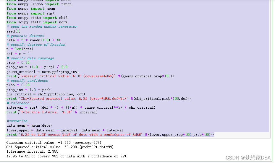
#parametric tolerance interval
from numpy.random import seed
from numpy.random import randn
from numpy import mean
from numpy import sqrt
from scipy.stats import chi2
from scipy.stats import norm
# seed the random number generator
seed(1)
# generate dataset
data = 5 * randn(100) + 50
# specify degress of freedom
n = len(data)
dof = n - 1
# specify data coverage
prop = 0.95
prop_inv = (1.0 - prop) / 2.0
gauss_critical = norm.ppf(prop_inv)
print('Gaussian critical value: %.3f (coverage=%d%%)' %(gauss_critical,prop*100))
# specify confidence
prob = 0.99
prop_inv = 1.0 - prob
chi_critical = chi2.ppf(prop_inv, dof)
print('Chi-Squared critical value: %.3f (prob=%d%%,dof=%d)' %(chi_critical,prob*100,dof))
# tolerance
interval = sqrt((dof * (1 + (1/n)) * gauss_critical**2) / chi_critical)
print('Tolerance Interval: %.3f' % interval)

#summarize
data_mean = mean(data)
lower,upper = data_mean - interval, data_mean + interval
print('%.2f to %.2f covers %d%% of data with a confidence of %d%%' %(lower,upper,prop*100,prob*100))

Running the example first calculates and prints the relevant critical values for the Gaussian and Chi-Squared distributions. The tolerance is printed, then presented correctly.

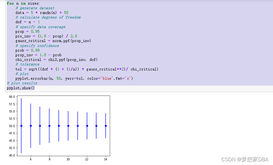
 It can also be helpful to demonstrate how the tolerance interval will decrease (become more precise) as the size of the sample is increased. The example below demonstrates this by calculating the tolerance interval for different sample sizes for the same small contrived problem.

 

# plot tolerance interval vs sample size
from numpy.random import seed
from numpy.random import randn
from numpy import sqrt
from scipy.stats import chi2
from scipy.stats import norm
from matplotlib import pyplot
# seed the random number generator
seed(1)
# sample sizes
seed(1)
#sample sizes
sizes = range(5,15)
for n in sizes:
    # generate dataset
    data = 5 * randn(n) + 50
    # calculate degrees of freedom
    dof = n - 1
    # specify data coverage
    prop = 0.95
    pro_inv = (1.0 - prop) / 2.0
    gauss_critical = norm.ppf(prop_inv)
    # specify confidence
    prob = 0.99
    prop_inv = 1.0 - prob
    chi_critical = chi2.ppf(prop_inv, dof)
    # tolerance
    tol = sqrt((dof * (1 + (1/n)) * gauss_critical**2)/ chi_critical)
    # plot
    pyplot.errorbar(n, 50, yerr=tol, color='blue',fmt='o')
# plot results
pyplot.show()

Running the example creates a plot showing the tolerance interval around the true population mean. We can see that the interval becomes smaller (more precise) as the sample size is increased from 5 to 15 examples.