1 Parameter estimation 、 Frequency school and Bayesian school
1.1 Maximum likelihood estimation
set up \(\bm{X}=(X_1,\dots X_n)\)( here \(\bm{X}\) It's a random vector , Refer to the sample , Note that the sample in machine learning is a single data point , In statistics, sample refers to the collection of all data ) Is from \(f(\bm{x}|\bm{\theta})\)(\(\bm{\theta}=(\theta_1,\dots,\theta_k)\)) Is the independent identically distributed population of its density function or probability mass function (iid) sample . If you observe \(\bm{X}=\bm{x}\), Then we define a conditional distribution called likelihood function \(L(\bm{\bm{\theta}}|\bm{X}) = f(\bm{X}|\bm{\bm{\theta}})\) To indicate when observation \(\bm{X}=\bm{x}\) when , Parameters \(\bm{\bm{\theta}}\) Probability distribution of .
Because the samples are independent and identically distributed , We have :
So for a fixed random vector \(\bm{x}\), Make \(\hat{\bm{\theta}}(x)\) Is the parameter \(\bm{\theta}\) A value of , It makes the \(L(\bm{\theta}|\bm{X})\) As \bm{\theta} Of The function reaches its maximum value here , Then based on the sample \(\bm{X}\) Maximum likelihood estimator of (maximum likelihood esitimator Abbreviation for MLE) Namely \(\hat{\bm{\theta}}(\bm{X})\).
And to make the likelihood function \(L(\bm{\theta}|\bm{X})\) Maximum , It is obviously an optimization problem , If the likelihood function is differentiable ( about \(\theta_i\)), that MLE The possible value of is to satisfy
Solution \((\theta_1, . . . , \theta_k)\). Note that the solution of this equation is only MLE Possible options for , Because the first derivative is \(0\) It is only a necessary but not sufficient condition to become the extreme point ( Plus the second-order condition we mentioned earlier ). in addition , The zero value of the first derivative is in the domain of function definition \(Ω\) On the internal extreme point ( That is, the inner point ). If the extreme point appears in the definition field \(Ω\) On the border of , The first derivative is not necessarily \(0\), Therefore, we must check the boundary to find the extreme point .
In general , When using differentiation , Handle \(L(\bm{\theta}|\bm{X})\) The natural logarithm of \(\text{log}(\bm{\theta}|\bm{X})\)( It is called logarithm Natural function ,log likelihood) Than direct processing \(L(\bm{\theta}|\bm{X})\) Easy to . This is because \(\text{log}\) It's a concave function ( Adding a minus sign is a convex function ), And is \((0, ∞)\) Strictly increasing function on , This implies \(L(\bm{\theta}|\bm{X})\) And \(\text{log}(\bm{\theta}|\bm{X})\) The extreme points of are consistent .
Let's take an example to demonstrate . The following example is very important , Later, we will make statistics in the learning column Logistic The regression is based on the enhanced version of this example . set up \(\bm{X}=(X_1,...X_n\)) yes iid Of , And the obedience parameter is \(p\) Of Bernoulli( Read as Bernoulli ) Distribution ( For students who forget Bernoulli distribution, see 《Python Random sampling and probability distribution in ( Two )》)), So the likelihood function is defined as :
Although the differentiation of this function is not particularly difficult , But log likelihood function
The differential of is very simple , We make \(L(p|\bm{X})\) Differential and let the result be 0, You get the solution :
So we have proved \(\sum X_i/n\) yes \(p\) Of MLE.
Of course , once \(L(p|\bm{X})\) Complicated , It is difficult for us to find the optimal solution analytically , So we're going to use 《 numerical optimization : First and second order optimization algorithms (Pytorch Realization )》 The gradient descent method learned 、 Newton method and other numerical optimization methods to find its numerical solution ( Because we are Is to maximize the likelihood function , The optimization algorithm is to minimize the function , Therefore, you should add a negative sign to the objective function when using ).
1.2 Bayesian estimation
The maximum likelihood estimation method is very classic , But there is another parameter estimation method that is significantly different from it , be called Bayes Method .( Be careful Bayes Method is a parameter estimation method , Stay with us 《 Statistical learning : Naive bayesian model (Numpy Realization )》 The Bayesian model is different , Don't get confused ) Some aspects of Bayesian method are quite helpful for other statistical methods .
In the classical maximum likelihood estimation method , Parameters \(θ\) Considered an unknown 、 But a fixed amount , From the \(θ\) As an indicator The overall Take a group of random samples from \(X_1,...X_n\), Obtain information about... Based on the observations of the sample \(θ\) Knowledge , People who hold this view are called Frequency school . stay Bayes In the method ,\(θ\) Is a change that can be one Quantity described by probability distribution , This distribution is called Prior distribution (prior distribution), This is a subjective distribution , Based on the experimenter's belief (belief) On , And it has been formulated with a formula before seeing the sampling data ( Therefore, it is called a priori ). Then from \(θ\) Take a group of samples from the population of the index , The prior distribution is corrected by the sample information , People who hold this view are called Bayesian school . This is called a positive prior distribution Posterior distribution (posterior distribution), This correction is called Bayes Statistics .
We record the prior distribution as \(π(θ)\) And record the sample distribution as \(f(\bm{x}|θ)\), Then the posterior distribution is a given sample \(\bm{x}\) Under the condition of \(θ\) The conditional distribution of , From Bayes formula :
Here's the denominator \(m(\bm{x})=\int f(\bm{x}|θ)π(θ)dθ\) yes \(\bm{X}\) The marginal distribution of .
Note that this posterior distribution is a conditional distribution , The condition is based on the observed samples . Now use this posterior distribution to make a decision about \(θ\) To infer , and \(θ\) It is still considered as a random quantity , What we get is its probability distribution , If you want to give a model , Usually take the model with the largest a posteriori probability . Besides , The mean of the posterior distribution can be used as \(θ\) Point estimate of .
Different from maximum likelihood estimation, numerical optimization is used to solve ,Bayes It is estimated that because it involves integral , We Numerical integration methods such as Monte Carlo are often used to solve .Although frequency school and Bayesian school have different understanding of Statistics , But you can simply connect the two Tie it up . We make \(D\) According to the data , about \(P(θ|D) = P(θ)P(D|θ)/P(D)\) Suppose the prior distribution is uniform , Take the maximum a posteriori probability , We can get the maximum likelihood estimation from Bayesian estimation . Next, Bayesian estimation and maximum likelihood estimation are compared :
Given data set \(D\), Maximum likelihood estimation :\(\hat{θ} = \underset{\theta}{\text{argmax}} P(D|θ)\)
Given data set \(D\), Bayesian estimation :\(\hat{P}(θ|D) =P(θ)P(D|θ)/P(D)\)
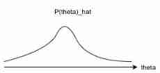 It can be seen that , The former is a point estimate , The latter gets a probability distribution .
 notes : A priori and a posteriori in philosophy
Human understanding of the objective world is divided into “ transcendental ” and “ Posttest ”. Posteriori refers to the knowledge generated by human experience , A priori refers to human beings' understanding of the objective world through their own rationality beyond experience .
In the past, philosophers had great differences on whether human beings' understanding of the objective world came from experience or rationality , It is also divided into two schools . One is Rationalism , Mainly based on Descartes of France 、 Leibniz of Germany is the representative , They believe that human beings can understand the world through their absolute rationality . Because the philosophers of this school are mainly from the European continent , So their theory is called “ European Philosophy ”. Another school is empiricism , Mainly represented by Hume of England , They believe that human beings can only know the world through experience . Hume is also an agnostic holder , He believes that human experience is unreliable , This makes the world unknowable to people .
Now it seems , The dispute between frequency school and Bayesian school is so similar to that between empiricism and rationalism !
Most machine learning models need to learn data sets “ Posttest ” Knowledge to get . Some people in academia believe that human knowledge is not acquired through acquired experience , Like music 、 literature 、 Drama generally needs innate talent or inspiration , Some scholars think it is “ transcendental ” Or is it “ Transcendental ” Of . Interestingly , According to Plato's cave man theory , Living in the world is like a cave man living in a cave , For example, cavers can only approximately recognize things outside the cave through the projection on the cave wall , Human beings can only approximately understand the abstract conceptual world through the things in the physical world , But can't fully understand it . Plato thought , music 、 Literature is something like existence Part of the conceptual world that lies in the abstract world , Human beings have been born in the abstract world , In the physical world, musicians 、 Writers are just trying their best to approximate these things , And it can never be completely reproduced .
obviously , According to the inference of Plato's view ,AI Learn mainly through experience , Nature can't understand the abstract world “ Rational formula ”. This is also for the purpose of AI Can play chess 、 Defeat humans in the game , And in music 、 Literature and other fields are difficult to surpass mankind, providing an explanation .
2 Estimate the variance and deviation of parameters
We can apply more than one method to estimate the parameters of probability distribution , This requires us to evaluate the quality of parameter estimators .
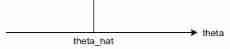
Parameters \(θ\) An estimate of \(W\) The mean square error of (mean squared error,MSE, Be careful : Here and me The application scenarios of the mean square error of the least squares in front of you are different , But ideas are similar ) By \(\mathbb{E}_θ(W-θ)^2\) Defined about \(θ\) Function of . Parameters \(θ\) Point estimator of \(W\) The deviation of (bias) It means \(W\) Our expectations are similar to \(θ\) The difference between the , namely \(\text{Bias}_θW=\mathbb{E}_θW-θ\). An estimator if its deviation ( About \(θ\)) The identity of is equal to 0, It is called a Unbiased (unbiased), It meets the \(\mathbb{E}_θW=θ\) For all \(θ\) establish . meanwhile , We also define estimators \(θ\) The variance of \(\text{Var}(W)\), The square root of the variance is called the standard deviation (standard error), Remember to do \(\text{SE}(W)\).
3 variance - Deviation decomposition and over fitting
such MSE Even all parameter estimates consist of two parts , Its degree is the variance of the estimator , Second, measure its deviation , namely
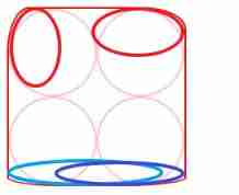
A good estimator should be small in variance and deviation . To get a good MSE nature We need to find the estimator whose variance and deviation are both controlled . Obviously, the unbiased estimator is right It's best to control the deviation .
For an unbiased estimator , We have :
If an estimator is unbiased , its MSE Is its variance .
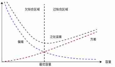
The relationship between deviation and variance and the capacity of machine learning model 、 The concepts of under fitting and over fitting are closely linked , use MSE Measure generalization error ( Both bias and variance are meaningful for generalization errors ) when , Increasing capacity increases variance , Reduce deviation . As shown in the figure below , This is called generalization error U Type curve .
quote
- [1] Calder K. Statistical inference[J]. New York: Holt, 1953.
- [2] expericnce . Statistical learning method ( The first 2 edition )[M]. tsinghua university press , 2019.
- [3] Ian Goodfellow,Yoshua Bengio etc. . Deep learning [M]. People's post and Telecommunications Press , 2017.
- [4] zhou . machine learning [M]. tsinghua university press , 2016.


![[DIY]自己设计微软MakeCode街机,官方开源软硬件](/img/a3/999c1d38491870c46f380c824ee8e7.png)