Using class weight to improve class imbalance

flutter + Applet + Back end ,3 Individuals can open your APP The way | Registration will be sent to Dajiang Yuntai 、 Huawei watch ！>>>

author |PROCRASTINATOR compile |VK source |Analytics Vidhya

summary

• Understand how class weight optimization works , And how to logistic Used in regression or any other algorithm sklearn Implement the same approach

• Learn how to... Without using any sampling method , By modifying the class weight, we can overcome the problem of class imbalance data

Introduce

The classification problem in machine learning is that we give some input （ Independent variables ）, And we have to predict a discrete target . The distribution of discrete values is likely to be very different . Because of the difference between each class , Algorithms tend to favor most of the existing values , But it is not good to deal with a few values .

This difference in class frequency affects the overall predictability of the model .

It's not difficult to get good accuracy on these questions , But that doesn't mean the model is good . We need to check whether the performance of these models has any commercial significance or value . That's why understanding problems and data is essential , So you can use the right metrics and optimize it in the right way .

Catalog

• What is category imbalance ？

• Why deal with category imbalances ？

• What is category weight ？

• logistic Class weight in regression

• Python Realization

  • Simple logistic Return to
  • weighting logistic Return to （' Balance '）
  • weighting logistic Return to （ Manual weights ）

• Skills to further improve your score

What is category imbalance ？

Class imbalance is a problem in machine learning classification . It only shows that the frequency of the target class is highly unbalanced , In other words, the frequency of one class is very high compared with other existing classes . let me put it another way , Bias against most of the classes in the target .

Suppose we consider a dichotomy , Most of these target classes have 10000 individual , A few target classes have only 100 individual . under these circumstances , The ratio is 100:1, That is, every 100 Most classes , There's only one minority . The problem is what we call class imbalance . The general areas where we can find this data are fraud detection 、 Loss prediction 、 Medical diagnosis 、 Email classification, etc .

We're going to deal with a data set in the field of Medicine , To correctly understand class imbalance . ad locum , We have to depend on the given properties （ Independent variables ） To predict whether a person will have a heart attack . To skip data cleaning and preprocessing , We're using a cleaned up version of the data .

In the image below , You can see the distribution of the target variables .

# Draw a bar chart of the target 
plt.figure(figsize=(10,6))
g = sns.barplot(data['stroke'], data['stroke'], palette='Set1', estimator=lambda x: len(x) / len(data) )

# Graph statistics 
for p in g.patches:
        width, height = p.get_width(), p.get_height()
        x, y = p.get_xy() 
        g.text(x+width/2, 
               y+height, 
               '{:.0%}'.format(height), 
               horizontalalignment='center',fontsize=15)

# Set the label 
plt.xlabel('Heart Stroke', fontsize=14)
plt.ylabel('Precentage', fontsize=14)
plt.title('Percentage of patients will/will not have heart stroke', fontsize=16)

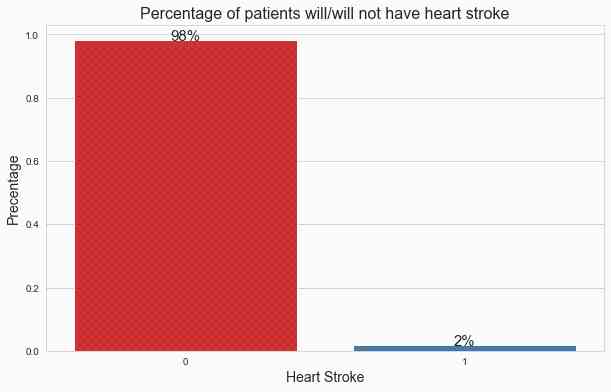
ad locum ,

0： It means that the patient has no heart disease .

1： The patient has a heart attack .

It can be seen from the distribution that , Only 2% Of the patients with heart disease . therefore , This is a classic category imbalance problem .

Why deal with category imbalances ？

up to now , We've got an intuitive sense of class imbalances . But why do we need to overcome this problem , What problems arise when modeling with these data ？

Most machine learning algorithms assume that the data is evenly distributed in the class . In the class imbalance problem , The broad problem is that the algorithm will be more inclined to predict most categories （ There is no heart disease in our case ）. The algorithm does not have enough data to learn a few classes （ heart disease ） The pattern in .

Let's take a real-life example to better understand this .

Suppose you have moved from your hometown to a new city , You lived here for a month . When you come to your hometown , You'll be very familiar with all the places , Like your home , Route , Important stores , Tourist attractions and so on , Because you spent your whole childhood there .

But in the new city , You don't think too much about the exact location of each place , The chance of getting lost on the wrong route is very high . ad locum , Your hometown is your majority , New towns are a minority .

Again , This can also happen in category imbalances . A few classes don't have enough information about your class , That's why a few classes have a high misclassification error .

notes ： To check the performance of the model , We will use f1 Score as a measure , Not accuracy .

The reason is that if we build a stupid model , Predict each new training data as 0（ No heart disease ）, Even so , We will also get very high accuracy , Because the model is biased towards most classes .

ad locum , The model is very accurate , But there's no value in our problem statement . That's why we're going to use f1 The score is used as the evaluation index .F1 The score is just a harmonic average of precision and recall . however , The metrics are chosen based on business issues and the types of errors we want to reduce . however ,f1 Score is the key to measure the problem of class imbalance .

Here are f1 The fraction formula ：

f1 score = 2*(precision*recall)/(precision+recall)

Let's confirm this by training a model based on the target variable pattern , And check the scores we get ：

# Training models with target patterns 
from sklearn.metrics import f1_score, accuracy_score, confusion_matrix
pred_test = []
for i in range (0, 13020):
    pred_test.append(y_train.mode()[0])

# Print f1 And accuracy scores 
print('The accuracy for mode model is:', accuracy_score(y_test, pred_test))
print('The f1 score for the model model is:',f1_score(y_test, pred_test))

# Draw confusion matrix 
conf_matrix(y_test, pred_test)

The accuracy of the pattern model is ：0.9819508448540707

Pattern pattern f1 The score is ：0.0

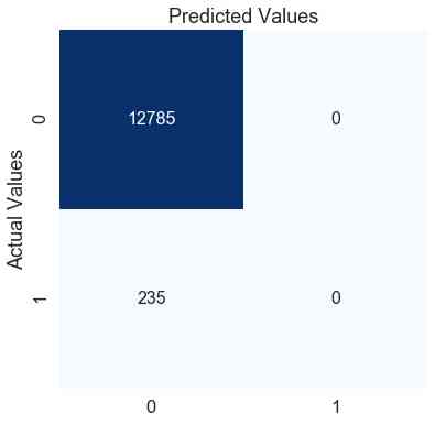
ad locum , The accuracy of the model to the test data is 0.98, It's a good score . But on the other hand ,f1 The score is zero , This shows that the model performs poorly in minority groups . We can confirm this by looking at the confusion matrix .

The model predicts that each patient is 0（ No heart disease ）. According to this model , No matter what kind of symptoms the patient has , He / She'll never have a heart attack . Does it make sense to use this model ？

Now we've learned what class imbalance is and how it affects our model performance , We're going to focus on what class weights are and how they help improve model performance .

What is the category weight ？

Most machine learning algorithms are not very useful for biased class data . however , We can modify the existing training algorithm , To take into account the skewed distribution of classes . This can be achieved by giving different weights to the majority and the minority categories . In the training phase , The difference of weight will affect the classification of categories . The overall goal is to set a higher class weight , At the same time, reduce the weight for most classes , To punish the wrong classification of a few classes .

To make this clearer , We're going to revert to the example of cities that we've considered before .

Think about it this way , You spent the last month in this new city , Instead of going out when you need to , It took a whole month to explore the city . You spend more time throughout the month learning about the routes and locations of the city . Giving you more time to study will help you better understand the new city , And reduce the chance of getting lost . This is how class weights work .

In the process of training , We give more weight to a few classes in the cost function of the algorithm , To enable it to provide higher penalties for a few classes , So that the algorithm can focus on reducing the error of a few classes .

Be careful ： There's a threshold , You should increase and decrease the class weight of the minority class and the majority class respectively . If you give a few classes a very high class weight , The algorithm is likely to favor a few classes , And it will increase errors in most classes .

majority sklearn Classifier modeling library , Some are even based on boosting The library of , Such as LightGBM and catboost, Each has a built-in parameter “class_weight”, This helps us optimize the scores for a few categories , As we've learned so far .

By default ,class_weights The value of is “None”, That is, the weight of the two classes is equal . besides , We can give it “balanced” Or pass in a dictionary containing the manually designed weights of two classes .

When the class weights =‘ Balance ’ when , The model will automatically assign class weights that are inversely proportional to their respective frequencies .

To be more precise , The formula is ：

wj=n_samples / (n_classes * n_samplesj)

ad locum ,

• wj Is the weight of each class （j Represents a class ）

• n_samples Is the total number of samples or rows in the dataset

• n_classes Is the total number of unique classes in the target

• n_samplesj Is the total number of rows of the corresponding class

For our heart case ：

n_samples= 43400, n_classes= 2(0&1), n_sample0= 42617, n_samples1= 783

0 Class weight ：

w0=  43400/(2*42617) = 0.509

1 Class weight ：

w1= 43400/(2*783) = 27.713

I hope this will make it clear that , Category weight =‘balanced’ It helps us give more weight to a few categories , Give most categories a lower weight .

Although in most cases , Take the value as “balanced” Delivery will produce good results , But sometimes for extreme classes it's unbalanced , We can try to design weights . We'll see how to do it later Python Find the best value of class weight in .

Logistic Class weight in regression

We can modify each machine learning algorithm by adding different class weights to the cost function of the algorithm , But here we will pay special attention to logistic Return to .

about logistic Return to , We use logarithmic loss as a cost function . We don't use mean square error as logistic Regression cost function , Because we use sigmoid Curve as a prediction function , Instead of fitting straight lines .

take sigmoid Function flattening results in a nonconvex curve , This makes the cost function have a large number of local minima , It is very difficult to converge to the global minimum by gradient descent method . But the logarithmic loss is a convex function , We have only one minimum that can converge .

log The loss formula ：

ad locum ,

• N It's the number of values

• yi Is the actual value of the target class

• yi Is the prediction probability of the target class

Let's form a pseudo table , It includes actual forecasts 、 Predict probability and use log The cost calculated by the loss formula ：

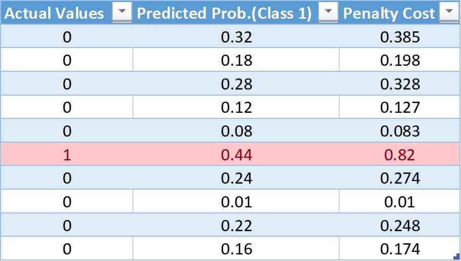
In this table , We have 10 Observations , among 9 One from 0 class ,9 One from 1 class . In the next column , We will give the probability of prediction for each observation . Last , Using the logarithmic loss formula , We get a cost penalty .

After adding the weight to the cost function , The modified logarithmic loss function is ：

here

w0 It's a class 0 Class weight of

w1 It's a class 1 Class weight of

Now? , We're going to add weights , See what effect it has on cost penalties .

For weight values , We will use class_weights='balanced' The formula .

w0= 10/(2*1) = 5

w1= 10/(2*9) = 0.55

Calculate the cost of the first value in the table ：

Cost = -(5(0*log(0.32) + 0.55(1-0)*log(1-0.32))

= -(0 + 0.55*log(.68))

= -(0.55*(-0.385))

= 0.211

Again , We can calculate the weighted cost of each observation , The updated table is ：

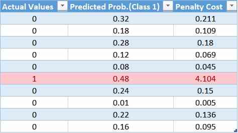
Through the table , We can be sure that a smaller weight is applied to the cost function of most classes , This leads to smaller error values , This reduces the updating of model coefficients . A larger weight value is applied to the cost function of a few classes , This leads to greater error calculations , Then the model coefficients are updated more . such , We can change the model bias , So as to reduce the error of a few classes .

Conclusion ：

Smaller weights result in smaller penalties and smaller updating of model coefficients

A larger weight will lead to a larger penalty and a large number of updates to the model coefficients

Python Realization

ad locum , We're going to use the same heart disease data to predict . First , We're going to train a simple logistic Return to , Then we're going to implement weighting logistic Return to , Class weight is “ Balance ”. Last , We'll try to use grid search to find the best value for class weights . The indicators we are trying to optimize will be f1 fraction .

1 Simple logical regression ：

here , We use sklearn Library to train our models , We use the default logistic Return to . By default , The algorithm will give equal weight to the two classes .

# Import and train models 
from sklearn.linear_model import LogisticRegression
lr = LogisticRegression(solver='newton-cg')
lr.fit(x_train, y_train)

# Test data prediction 
pred_test = lr.predict(x_test)

# Calculate and print f1 fraction 
f1_test = f1_score(y_test, pred_test)
print('The f1 score for the testing data:', f1_test)

#  Function to create confusion matrix 
def conf_matrix(y_test, pred_test):    
    
    #  Create confusion matrix 
    con_mat = confusion_matrix(y_test, pred_test)
    con_mat = pd.DataFrame(con_mat, range(2), range(2))
   
    plt.figure(figsize=(6,6))
    sns.set(font_scale=1.5) 
    sns.heatmap(con_mat, annot=True, annot_kws={"size": 16}, fmt='g', cmap='Blues', cbar=False)
    
# Call function 
conf_matrix(y_test, pred_test)

Test data f1 score ：0.0

In simple logistic In the regression model ,f1 The score is 0. By observing the confusion matrix , We can confirm that our model predicts every observation , Because there's no heart attack . This model is no better than the pattern model we created earlier . Let's try to add some weight to a few classes , See if it helps .

2 Logical regression （class_weight='balanced'）：

We are logistic The class weight parameter is added to the regression algorithm , The value passed is “balanced”.

# Import and train models 
from sklearn.linear_model import LogisticRegression
lr = LogisticRegression(solver='newton-cg', class_weight='balanced')
lr.fit(x_train, y_train)

#  Test data prediction 
pred_test = lr.predict(x_test)

#  Calculate and print f1 fraction 
f1_test = f1_score(y_test, pred_test)
print('The f1 score for the testing data:', f1_test)

# Draw confusion matrix 
conf_matrix(y_test, pred_test)

Test data f1 score ：0.10098851188885921

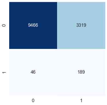
By means of logistic Add a single weight parameter to the regression function , We will f1 The score has improved 10%. We can see in the confusion matrix , Although class 0（ No heart disease ） The misclassification of has been increased , But models can capture classes well 1（ heart disease ）.

Can we further improve metrics by changing the class weight ？

3 Logical regression （ Manually set the class weight ）：

Last , We try to use grid search to find the best weight with the highest score . We will search for 0 To 1 Between the weight of . Our idea is , If we give a few categories n As weights , Most categories will get 1-n As weights .

ad locum , The weight is not very big , But the weight ratio between most categories and a few categories will be very high .

for example ：

w1 = 0.95

w0 = 1 – 0.95 = 0.05

w1:w0 = 19:1

therefore , The weight of a few categories will be that of the majority 19 times .

from sklearn.model_selection import GridSearchCV, StratifiedKFold
lr = LogisticRegression(solver='newton-cg')

# Set the range of class weight 
weights = np.linspace(0.0,0.99,200)

# Create a dictionary grid for grid search 
param_grid = {'class_weight': [{0:x, 1:1.0-x} for x in weights]}

## use 5 The double grid search method is used to fit the training data 
gridsearch = GridSearchCV(estimator= lr, 
                          param_grid= param_grid,
                          cv=StratifiedKFold(), 
                          n_jobs=-1, 
                          scoring='f1', 
                          verbose=2).fit(x_train, y_train)

# Draw scores with different weight values 
sns.set_style('whitegrid')
plt.figure(figsize=(12,8))
weigh_data = pd.DataFrame({ 'score': gridsearch.cv_results_['mean_test_score'], 'weight': (1- weights)})
sns.lineplot(weigh_data['weight'], weigh_data['score'])
plt.xlabel('Weight for class 1')
plt.ylabel('F1 score')
plt.xticks([round(i/10,1) for i in range(0,11,1)])
plt.title('Scoring for different class weights', fontsize=24)

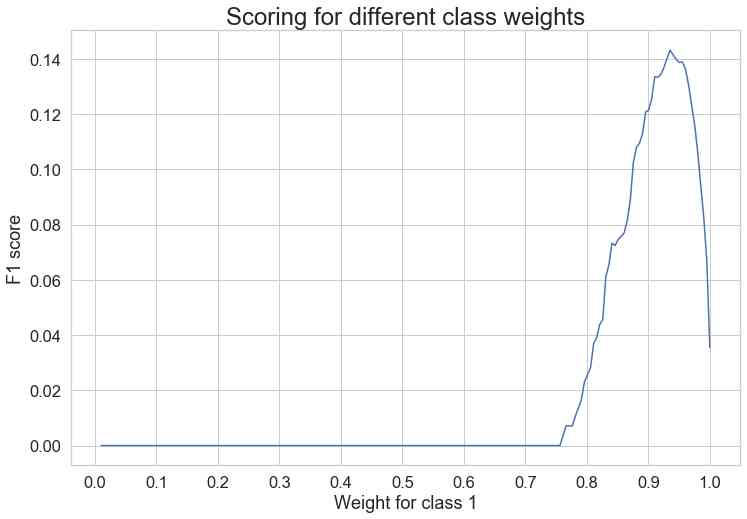
From the graph, we can see that the highest value of a few classes is in 0.93 It's peaking at .

Search through the grid , We get the best class weight ,0 class （ Most classes ） by 0.06467,1 class （ A few categories ） by 1:0.93532.

Now we have used hierarchical cross validation and grid search to get the best class weight , We'll see the performance of the test data .

# Import and train models 
from sklearn.linear_model import LogisticRegression
lr = LogisticRegression(solver='newton-cg', class_weight={0: 0.06467336683417085, 1: 0.9353266331658292})
lr.fit(x_train, y_train)

#  Test data prediction 
pred_test = lr.predict(x_test)

#  Calculate and print f1 fraction 
f1_test = f1_score(y_test, pred_test)
print('The f1 score for the testing data:', f1_test)

#  Draw confusion matrix 
conf_matrix(y_test, pred_test)

f1 fraction ：0.15714644

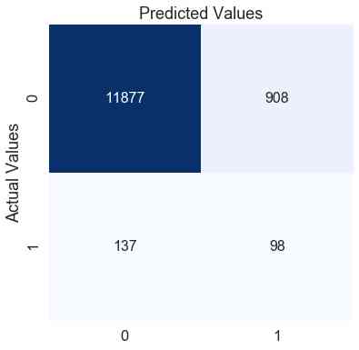
By manually changing the weight value , We can further improve f1 The score is about 6%. The confusion matrix also shows that , From the previous model , We can better predict 0 class , But the price is ours 1 Class error classification . It all depends on the business problem or the type of errors you want to reduce . ad locum , Our focus is on improving f1 fraction , We can do this by adjusting the weight of categories .

Further improve your scoring skills

Feature Engineering ： For the sake of simplicity , We only use the given arguments . You can try to create new features

Adjust the threshold ： By default , The threshold of all algorithms is 0.5. You can try different threshold values , And you can find the best value by using grid search or randomization search

Using advanced algorithms ： For this explanation , We only used logistic Return to . You can try different bagging and boosting Algorithm . Finally, we can try to mix a variety of algorithms

ending

I hope this article will give you an idea of how class weights help deal with class imbalances , And in python How easy it is to implement it in .

We have discussed how to use class weights only logistic Return to , But the idea of other algorithms is the same ; It's just the cost function changes that each algorithm uses to minimize errors and optimize a small number of results

Link to the original text ：https://www.analyticsvidhya.com/blog/2020/10/improve-class-imbalance-class-weights/

Welcome to join us AI Blog station ： http://panchuang.net/

sklearn Machine learning Chinese official documents ： http://sklearn123.com/

Welcome to pay attention to pan Chuang blog resource summary station ： http://docs.panchuang.net/