Outlier detection based on RNN self encoder

flutter + Applet + Back end ,3 Individuals can open your APP The way | Registration will be sent to Dajiang Yuntai 、 Huawei watch ！>>>

author |David Woroniuk compile |VK source |Towards Data Science

What is an anomaly

abnormal , Usually called outliers , Data points in the data that do not conform to the overall behavior of the data series 、 A sequence or pattern of data . therefore , Anomaly detection is the task of detecting data points or sequences that do not conform to patterns in a wider range of data .

Effective detection and deletion of abnormal data is very useful for many business functions , Such as detecting broken links embedded in the website 、 Peak Internet traffic or dramatic changes in stock prices . Mark these phenomena as outliers , Or develop a pre planned response , It can save enterprise time and money .

Exception types

Usually , Abnormal data can be divided into three categories ： Additive outliers 、 Abnormal value of time change or level change .

Additive outliers Is characterized by a sudden sharp increase or decrease in value , This may be driven by exogenous or endogenous factors . An example of an additive outlier may be a substantial increase in website traffic due to the emergence of TV programs （ External cause ）, Or a short-term increase in stock trading volume due to strong quarterly results （ Internal cause ）.

Time variation outliers Is characterized by a short sequence , It's not in line with the broader trends in the data . for example , If a web server crashes , On a series of data points , Website traffic will drop to zero , Until the server restarts , At this point, the flow will return to normal .

Abnormal value of horizontal change It's a common phenomenon in commodity markets , Because the high demand for electricity in the commodity market is intrinsically linked to bad weather conditions . So we can observe the difference between summer and winter electricity prices “ Level change ”, This is due to weather driven changes in demand and renewable energy generation .

What is a self encoder

An automatic encoder is a neural network designed to learn a low dimensional representation of a given input . An automatic encoder usually consists of two parts ： An encoder learns to map input data to low dimensional representations , Another decoder learns to map the representation back to the input data .

Because of this structure , The encoder network iteratively learns an efficient data compression function , This function maps data to a low dimensional representation . After training , The decoder can successfully reconstruct the original input data , Reconstruction error （ The difference between the input produced by the decoder and the reconstructed output ） It's the objective function of the whole training process .

Realization

Now that we understand the underlying architecture of the automatic encoder model , We can start to implement the model .

The first step is to install the library we will use 、 Packages and modules ：

#  Data processing :
import numpy as np
import pandas as pd
from datetime import date, datetime

# RNN Self encoder :
from tensorflow import keras
from tensorflow.keras import layers

#  mapping :
!pip install chart-studio
import plotly.graph_objects as go

secondly , We need to get some data to analyze . This article uses the historical encryption software package to obtain 2013 year 6 month 6 Bitcoin historical data from now on . The following code also generates the daily bitcoin rate of return and intraday price volatility , Then delete any missing data rows and return to the front of the data frame 5 That's ok .

#  Import  Historic Crypto  package :
!pip install Historic-Crypto
from Historic_Crypto import HistoricalData

#  Get bitcoin data , Calculate earnings and intraday volatility :
dataset = HistoricalData(start_date = '2013-06-06',ticker = 'BTC').retrieve_data()
dataset['Returns'] = dataset['Close'].pct_change()
dataset['Volatility'] = np.abs(dataset['Close']- dataset['Open'])
dataset.dropna(axis = 0, how = 'any', inplace = True)
dataset.head()

Now that we've got some data , We should visually scan each sequence for potential outliers . Below plot_dates_values The function iterates to draw each sequence contained in the data frame .

def plot_dates_values(data_timestamps, data_plot):
  '''
   This function provides a plan of the input sequence 
  Arguments: 
          data_timestamps:  The timestamp associated with each data instance .
          data_plot:  The sequence of data to plot .
  Returns:
          fig:  Use sliders and buttons to display the sequence of graphics .
  '''

  fig = go.Figure()
  fig.add_trace(go.Scatter(x = data_timestamps, y = data_plot,
                           mode = 'lines',
                           name = data_plot.name,
                           connectgaps=True))
  fig.update_xaxes(
    rangeslider_visible=True,
    rangeselector=dict(
        buttons=list([
            dict(count=1, label="YTD", step="year", stepmode="todate"),
            dict(count=1, label="1 Years", step="year", stepmode="backward"),
            dict(count=2, label="2 Years", step="year", stepmode="backward"),
            dict(count=3, label="3 Years", step="year", stepmode="backward"),
            dict(label="All", step="all")
        ]))) 
  
  fig.update_layout(
    title=data_plot.name,
    xaxis_title="Date",
    yaxis_title="",
    font=dict(
        family="Arial",
        size=11,
        color="#7f7f7f"
    ))
  return fig.show()

We can now call the above functions repeatedly , The volume of transactions that generate bitcoin 、 Closing price 、 Opening price 、 Volatility and yield curves .

plot_dates_values(dataset.index, dataset['Volume'])

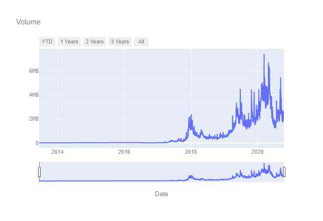
It is worth noting that ,2020 There were some peaks in trading volume in the year , It may be useful to investigate whether these peaks are abnormal or indicate a broader sequence .

plot_dates_values(dataset.index, dataset['Close'])

.png)

2018 There was an obvious rise in the closing price of the year , Then it fell to the level of technical support . However , An upward trend is prevalent throughout the data .

plot_dates_values(dataset.index, dataset['Open'])

.png)

The daily opening price is similar to the above closing price .

plot_dates_values(dataset.index, dataset['Volatility'])

.png)

2018 The price and volatility of the year are obvious . therefore , We can study whether these volatility peaks are considered abnormal by the auto encoder model .

plot_dates_values(dataset.index, dataset['Returns'])

.png)

Because of the randomness of the income series , We choose to test the outliers in the daily trading volume of bitcoin , Characterized by trading volume .

therefore , We can start data preprocessing for the automatic encoder model . The first step in data preprocessing is to determine the appropriate segmentation between training data and test data . As outlined below generate_train_test_split The function can split training and test data by date . When calling the following function , Two data frames will be generated , That is, training data and test data as global variables .

def generate_train_test_split(data, train_end, test_start):
  '''
   This function decomposes the data set into training data and test data by using strings . As 'train_end' and 'test_start' The string provided by the parameter must be consecutive days .
  Arguments: 
          data:  The data is divided into training data and test data .
          train_end:  Training data end date (str).
          test_start:  Test data start date (str).
  Returns:
          training_data:  Data used in model training (Pandas DataFrame).
          testing_data:  Data used in model testing (panda DataFrame).
  '''
  if isinstance(train_end, str) is False:
    raise TypeError("train_end argument should be a string.")
  
  if isinstance(test_start, str) is False:
    raise TypeError("test_start argument should be a string.")

  train_end_datetime = datetime.strptime(train_end, '%Y-%m-%d')
  test_start_datetime = datetime.strptime(test_start, '%Y-%m-%d')
  while train_end_datetime >= test_start_datetime:
    raise ValueError("train_end argument cannot occur prior to the test_start argument.")
  while abs((train_end_datetime - test_start_datetime).days) > 1:
    raise ValueError("the train_end argument and test_start argument should be seperated by 1 day.")

  training_data = data[:train_end]
  testing_data = data[test_start:]

  print('Train Dataset Shape:',training_data.shape)
  print('Test Dataset Shape:',testing_data.shape)

  return training_data, testing_data


#  We now call the above function , Generate training and test data 
training_data, testing_data = generate_train_test_split(dataset, '2018-12-31','2019-01-01')

In order to improve the accuracy of the model , We can do... On the data “ Standardization ” Or zoom . This function can scale the training data frame generated above , Keep training averages and training standards , In order to standardize the test data in the future .

notes ： It's important to scale training and test data at the same level , Otherwise, differences in scale will lead to interpretability problems and model inconsistencies .

def normalise_training_values(data):
  '''
   This function normalizes the input values with the mean and standard deviation .
  Arguments: 
          data:  To be standardized DataFrame Column .
  Returns:
          values:  Normalized data for model training (numpy Array ).
          mean:  Training set mean, For standardized test sets (float).
          std:  The standard deviation of the training set , For standardized test sets (float).
  '''
  if isinstance(data, pd.Series) is False:
    raise TypeError("data argument should be a Pandas Series.")

  values = data.to_list()
  mean = np.mean(values)
  values -= mean
  std = np.std(values)
  values /= std
  print("*"*80)
  print("The length of the training data is: {}".format(len(values)))
  print("The mean of the training data is: {}".format(mean.round(2)))
  print("The standard deviation of the training data is {}".format(std.round(2)))
  print("*"*80)
  return values, mean, std


#  Now call the function above :
training_values, training_mean, training_std = normalise_training_values(training_data['Volume'])

As we said above normalise_training_values function , We have one now numpy Array , It contains what is called training_values Standardized training data for , We have already training_mean and training_std Store as global variable , For standardized test sets .

We can now start generating a series of sequences , These sequences can be used to train the automatic encoder model . We define the window size 30, Providing a shape of 3D Training data (2004,30,1):

#  Define the number of time steps for each sequence :
TIME_STEPS = 30

def generate_sequences(values, time_steps = TIME_STEPS):
  '''
   This function generates a sequence of lengths to be passed to the model 'TIME_STEPS'.
  Arguments: 
          values:  Generating sequences (numpy Array ) The normalized value of .
          time_steps:  The length of the sequence (int).
  Returns:
          train_data:  For model training 3D data (numpy array).
  '''
  if isinstance(values, np.ndarray) is False:
    raise TypeError("values argument must be a numpy array.")
  if isinstance(time_steps, int) is False:
    raise TypeError("time_steps must be an integer object.")

  output = []

  for i in range(len(values) - time_steps):
    output.append(values[i : (i + time_steps)])
  train_data = np.expand_dims(output, axis =2)
  print("Training input data shape: {}".format(train_data.shape))

  return train_data
  
#  Now call the function above to generate x_train:
x_train = generate_sequences(training_values)

Now we have finished processing the training data , We can define the automatic encoder model , Then fit the model to the training data .define_model The function uses the shape of the training data to define the appropriate model , Returns a summary of the self encoder model and the self encoder model .

def define_model(x_train):
  '''
   This function uses x_train To generate RNN Model .
  Arguments: 
          x_train:  For model training 3D data (numpy array).
  Returns:
          model:  Model architecture (Tensorflow object ).
          model_summary:  A summary of the model architecture .
  '''

  if isinstance(x_train, np.ndarray) is False:
    raise TypeError("The x_train argument should be a 3 dimensional numpy array.")

  num_steps = x_train.shape[1]
  num_features = x_train.shape[2]

  keras.backend.clear_session()
  
  model = keras.Sequential(
      [
       layers.Input(shape=(num_steps, num_features)),
       layers.Conv1D(filters=32, kernel_size = 15, padding = 'same', data_format= 'channels_last',
                     dilation_rate = 1, activation = 'linear'),
       layers.LSTM(units = 25, activation = 'tanh', name = 'LSTM_layer_1',return_sequences= False),
       layers.RepeatVector(num_steps),
       layers.LSTM(units = 25, activation = 'tanh', name = 'LSTM_layer_2', return_sequences= True),
       layers.Conv1D(filters = 32, kernel_size = 15, padding = 'same', data_format = 'channels_last',
                     dilation_rate = 1, activation = 'linear'),
       layers.TimeDistributed(layers.Dense(1, activation = 'linear'))
      ]
  )

  model.compile(optimizer=keras.optimizers.Adam(learning_rate = 0.001), loss = "mse")
  return model, model.summary()

And then ,model_fit Function calls internally define_model function , And then provide the model with epochs、batch_size and validation_loss Parameters . And then call this function. , Start the model training process .

def model_fit():
  '''
   This function calls the above 'define_model()' function , And then according to x_train Data train the model .
  Arguments: 
          N/A.
  Returns:
          model:  Trained models .
          history:  A summary of how models are trained ( Training mistakes , Validation error ).
  '''
  #  stay x_train Use the above define_model function :
  model, summary = define_model(x_train)

  history = model.fit(
    x_train,
    x_train,
    epochs=400,
    batch_size=128,
    validation_split=0.1,
    callbacks=[keras.callbacks.EarlyStopping(monitor="val_loss", 
                                              patience=25, 
                                              mode="min", 
                                              restore_best_weights=True)])
  
  return model, history


#  Call the function above , Generating models and the history of models :
model, history = model_fit()

Once the model is trained , You have to draw training and validation loss curves , To see if there is any deviation in the model （ Under fitting ） Or variance （ Over fitting ）. This can be done by calling the following plot_training_validation_loss Function to observe .

def plot_training_validation_loss():
  '''
   This function draws the training and validation loss curves of the training model , Visual diagnosis can be made for under fitting or over fitting .
  Arguments: 
          N/A.
  Returns:
          fig: Visual representation of training loss and validation of the model 
  '''
  training_validation_loss = pd.DataFrame.from_dict(history.history, orient='columns')

  fig = go.Figure()
  fig.add_trace(go.Scatter(x = training_validation_loss.index, y = training_validation_loss["loss"].round(6),
                           mode = 'lines',
                           name = 'Training Loss',
                           connectgaps=True))
  fig.add_trace(go.Scatter(x = training_validation_loss.index, y = training_validation_loss["val_loss"].round(6),
                           mode = 'lines',
                           name = 'Validation Loss',
                           connectgaps=True))
  
  fig.update_layout(
  title='Training and Validation Loss',
  xaxis_title="Epoch",
  yaxis_title="Loss",
  font=dict(
        family="Arial",
        size=11,
        color="#7f7f7f"
    ))
  return fig.show()


#  Call the function above :
plot_training_validation_loss()

.png)

It is worth noting that , The training and validation loss curves converge throughout the chart , The verification loss is still slightly greater than the training loss . In the case of given shape error and relative error , We can confirm that there is no under fitting or over fitting in the automatic encoder model .

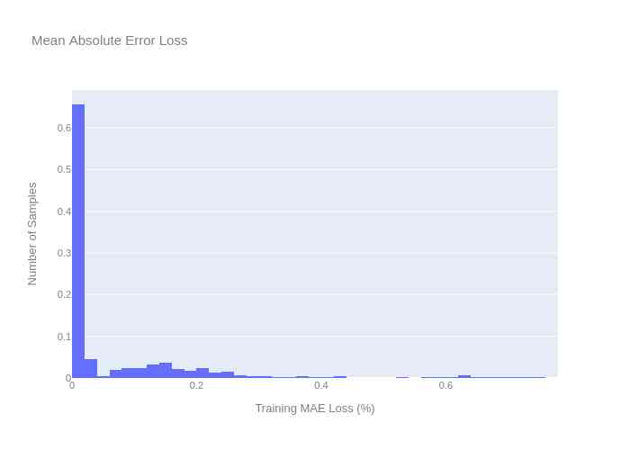
Now? , We can define the reconstruction error , This is one of the core principles of the automatic encoder model . Reconstruction errors are expressed as training losses , The reconstruction error threshold is the maximum training loss . therefore , In calculating the test error , Any value greater than the maximum training loss can be regarded as an abnormal value .

def reconstruction_error(x_train):
  '''
   This function calculates the reconstruction error , And display the histogram of training average absolute error 
  Arguments: 
          x_train:  For model training 3D data (numpy array).
  Returns:
          fig:  Training MAE Visualization of distribution .
  '''

  if isinstance(x_train, np.ndarray) is False:
    raise TypeError("x_train argument should be a numpy array.")

  x_train_pred = model.predict(x_train)
  global train_mae_loss
  train_mae_loss = np.mean(np.abs(x_train_pred - x_train), axis = 1)
  histogram = train_mae_loss.flatten() 
  fig =go.Figure(data = [go.Histogram(x = histogram, 
                                      histnorm = 'probability',
                                      name = 'MAE Loss')])  
  fig.update_layout(
  title='Mean Absolute Error Loss',
  xaxis_title="Training MAE Loss (%)",
  yaxis_title="Number of Samples",
  font=dict(
        family="Arial",
        size=11,
        color="#7f7f7f"
    ))
  
  print("*"*80)
  print("Reconstruction error threshold: {} ".format(np.max(train_mae_loss).round(4)))
  print("*"*80)
  return fig.show()


#  Call the function above :
reconstruction_error(x_train)

on top , We will training_mean and training_std Save as global variable , So that they can be used to scale test data . We now define normalise_testing_values Function to scale the test data .

def normalise_testing_values(data, training_mean, training_std):
  '''
   The function uses the training average and standard deviation to normalize the test data , To generate a test value numpy Array .
  Arguments: 
          data:  Data used (panda DataFrame Column )
          mean:  Training set average ( Floating point numbers ).
          std:   Training set standard deviation (float).
  Returns:
          values:  Array  (numpy array).
  '''
  if isinstance(data, pd.Series) is False:
    raise TypeError("data argument should be a Pandas Series.")

  values = data.to_list()
  values -= training_mean
  values /= training_std
  print("*"*80)
  print("The length of the testing data is: {}".format(data.shape[0]))
  print("The mean of the testing data is: {}".format(data.mean()))
  print("The standard deviation of the testing data is {}".format(data.std()))
  print("*"*80)

  return values

And then , stay testing_data Of Volume Call this function on the column . therefore ,test_value Be embodied as numpy Array .

#  Call the function above :
test_value = normalise_testing_values(testing_data['Volume'], training_mean, training_std) 

On this basis , The generation test loss function is defined , The difference between the reconstructed data and the test data is calculated . If any value is greater than the maximum training loss , Store it in the global exception list .

def generate_testing_loss(test_value):
  '''
   This function uses the model to predict anomalies in the test set . Besides , This function generates “ abnormal ” Global variables , Include by RNN Identified outliers .
  Arguments: 
          test_value:  Array of tests (numpy Array ).
  Returns:
          fig:  Training MAE Visualization of distribution .
  '''
  x_test = generate_sequences(test_value)
  print("*"*80)
  print("Test input shape: {}".format(x_test.shape))

  x_test_pred = model.predict(x_test)
  test_mae_loss = np.mean(np.abs(x_test_pred - x_test), axis = 1)
  test_mae_loss = test_mae_loss.reshape((-1))

  global anomalies
  anomalies = (test_mae_loss >= np.max(train_mae_loss)).tolist()
  print("Number of anomaly samples: ", np.sum(anomalies))
  print("Indices of anomaly samples: ", np.where(anomalies))
  print("*"*80)

  histogram = test_mae_loss.flatten() 
  fig =go.Figure(data = [go.Histogram(x = histogram, 
                                      histnorm = 'probability',
                                      name = 'MAE Loss')])  
  fig.update_layout(
  title='Mean Absolute Error Loss',
  xaxis_title="Testing MAE Loss (%)",
  yaxis_title="Number of Samples",
  font=dict(
        family="Arial",
        size=11,
        color="#7f7f7f"
    ))
  
  return fig.show()


#  Call the function above :
generate_testing_loss(test_value)

Besides , It also introduces MAE The distribution of , And with MAE The direct losses are compared .

.png)

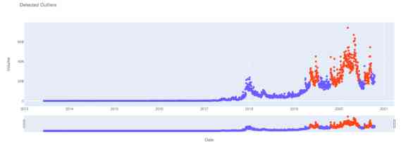
Last , The outliers are visually represented below .

def plot_outliers(data):
  '''
   This function determines the location of outliers in the time series , These outliers are plotted in turn .
  Arguments: 
          data:  Initial data set (Pandas DataFrame).
  Returns:
          fig:  from RNN A visual representation of outliers in a given sequence .
  '''

  outliers = []

  for data_idx in range(TIME_STEPS -1, len(test_value) - TIME_STEPS + 1):
    time_series = range(data_idx - TIME_STEPS + 1, data_idx)
    if all([anomalies[j] for j in time_series]):
      outliers.append(data_idx + len(training_data))

  outlying_data = data.iloc[outliers, :]

  cond = data.index.isin(outlying_data.index)
  no_outliers = data.drop(data[cond].index)

  fig = go.Figure()
  fig.add_trace(go.Scatter(x = no_outliers.index, y = no_outliers["Volume"],
                           mode = 'markers',
                           name = no_outliers["Volume"].name,
                           connectgaps=False))
  fig.add_trace(go.Scatter(x = outlying_data.index, y = outlying_data["Volume"],
                           mode = 'markers',
                           name = outlying_data["Volume"].name + ' Outliers',
                           connectgaps=False))
  
  fig.update_xaxes(rangeslider_visible=True)

  fig.update_layout(
  title='Detected Outliers',
  xaxis_title=data.index.name,
  yaxis_title=no_outliers["Volume"].name,
  font=dict(
        family="Arial",
        size=11,
        color="#7f7f7f"
    ))
  
  
  return fig.show()


#  Call the function above :
plot_outliers(dataset)

Remote data characterized by the automatic encoder model is represented in orange , Consistency data is shown in blue .

.png)

We can see ,2020 A large part of the annual bitcoin trading volume data is considered abnormal —— It may be due to Covid-19 Increased retail trading activity driven by ？

Try automatic encoder parameters and new data sets , See if you can find any anomalies in bitcoin's closing price , Or use the historical encryption library to download different cryptocurrencies ！

Link to the original text ：https://towardsdatascience.com/outlier-detection-with-rnn-autoencoders-b82e2c230ed9

Welcome to join us AI Blog station ： http://panchuang.net/

sklearn Machine learning Chinese official documents ： http://sklearn123.com/

Welcome to pay attention to pan Chuang blog resource summary station ： http://docs.panchuang.net/