当前位置:网站首页>Skimage learning (2) -- RGB to grayscale, RGB to HSV, histogram matching
Skimage learning (2) -- RGB to grayscale, RGB to HSV, histogram matching
2022-07-07 17:02:00 【Original knowledge】
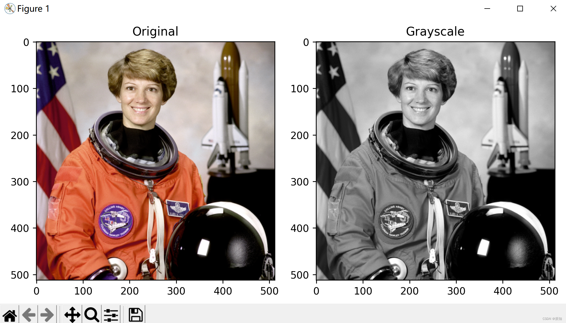
1、RGB Go gray
This example will have RGB The image of the channel is converted into an image with a single gray channel .
The value of each gray pixel is calculated as the corresponding red 、 Weighted sum of green and blue pixels :
Y = 0.2125 R + 0.7154 G + 0.0721 B
CRT Phosphors use these weights , Because they are more representative of human beings to red than the same weight 、 The perception of green and blue .
import matplotlib.pyplot as plt

from skimage import data
from skimage.color import rgb2gray

original = data.astronaut()
grayscale = rgb2gray(original)
#fig It's a variable name ,fig Represents the drawing window (Figure);ax Represents the coordinate system on this drawing window (axis), Will generally continue to ax To operate
# among figsize Used to set the size of the drawing ,a Is the width of the figure , b Is the height of the figure , In inches .
fig, axes = plt.subplots(1, 2, figsize=(8, 4))
ax = axes.ravel()

ax[0].imshow(original)
ax[0].set_title("Original")
ax[1].imshow(grayscale, cmap=plt.cm.gray)
ax[1].set_title("Grayscale")

fig.tight_layout()#ight_layout The subgraph parameters will be automatically adjusted , Make it fill the entire image area . This is an experimental feature , May not work in some cases . It just checks the axis labels 、 Scale label and title section .
plt.show()
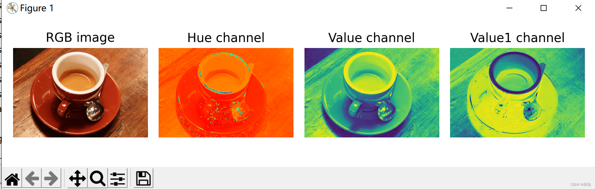
2、RGB turn HSV
hsv Detailed explanation :https://blog.csdn.net/bamboocan/article/details/70627137
This example shows how RGB To HSV( tonal , saturation , brightness ) Transformation can be used to facilitate the segmentation process .
Usually , The objects in the image have different colors ( tonal ) And brightness , So these features can be used to separate different areas of the image .
stay RGB In the middle , Hue and brightness are expressed as R、G、B Linear combination of channels , And they correspond to HSV Single channel of image ( Hue and value channels ).
A simple segmentation image , Then, threshold only HSV passageway .
For example, picture dyeing homogenization , We often use rgb2hsv To solve the problem , It can effectively protect the texture 、 Distribution and other characteristics .
Here we look at an example of chromosome color separation :
Be careful , The example here is HED Color space ,HSV Space is the same effect .
from skimage import io
import matplotlib.pyplot as plt
import matplotlib.pyplot as plt
from skimage import data
from skimage.color import rgb2hsv
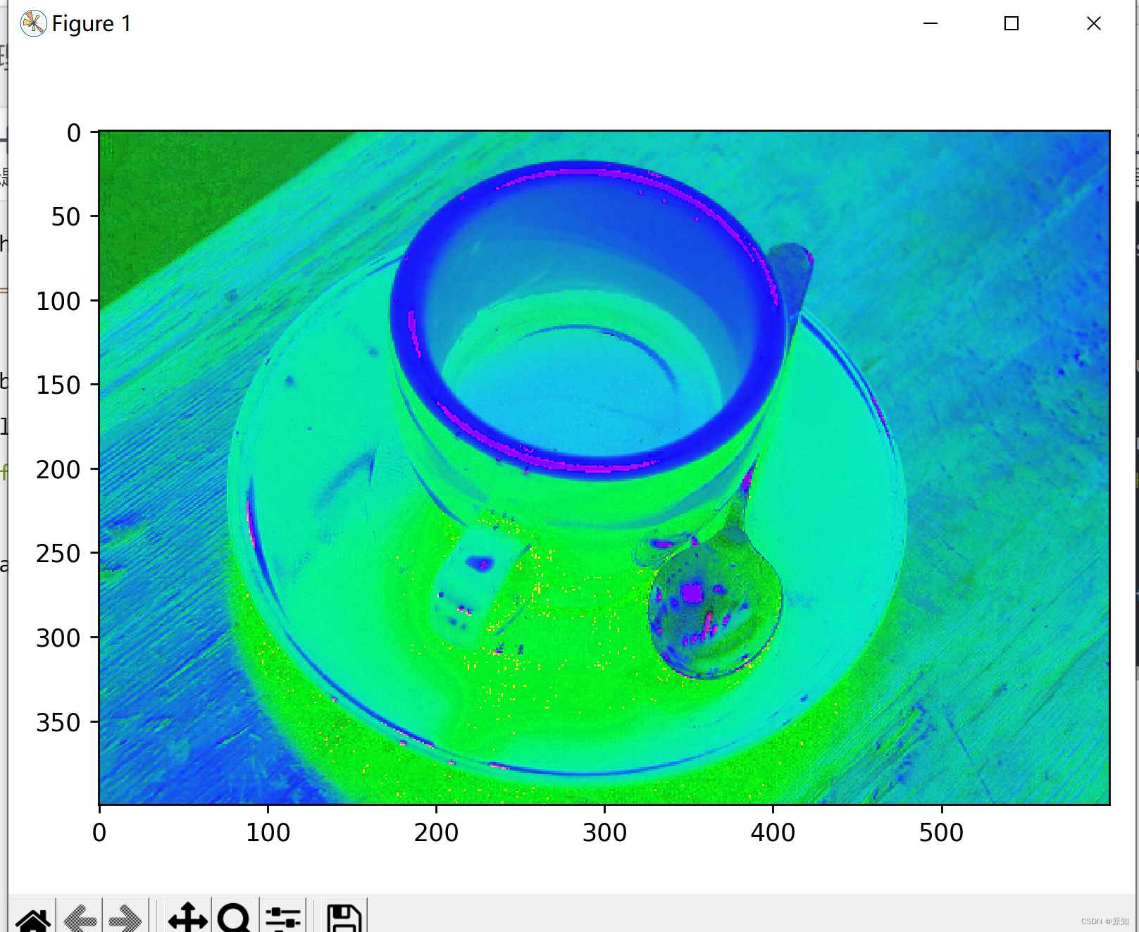
# First load RGB Image and extract Hue and Value passageway :
rgb_img = data.coffee()
hsv_img = rgb2hsv(rgb_img)
io.imshow(hsv_img)
plt.show()
hue_img = hsv_img[:, :, 0]# It is a way to process multidimensional data , It represents the first two dimensions , Take all of them 0 Index number .
value_img = hsv_img[:, :, 2]
value1_img = hsv_img[:, :, 1]
fig, (ax0, ax1, ax2,ax3) = plt.subplots(ncols=4, figsize=(8, 2))
ax0.imshow(rgb_img)
ax0.set_title("RGB image")
ax0.axis('off')
ax1.imshow(hue_img, cmap='hsv')
ax1.set_title("Hue channel")
ax1.axis('off')
ax2.imshow(value_img)
ax2.set_title("Value channel")
ax2.axis('off')
ax3.imshow(value1_img)
ax3.set_title("Value1 channel")
ax3.axis('off')
fig.tight_layout()
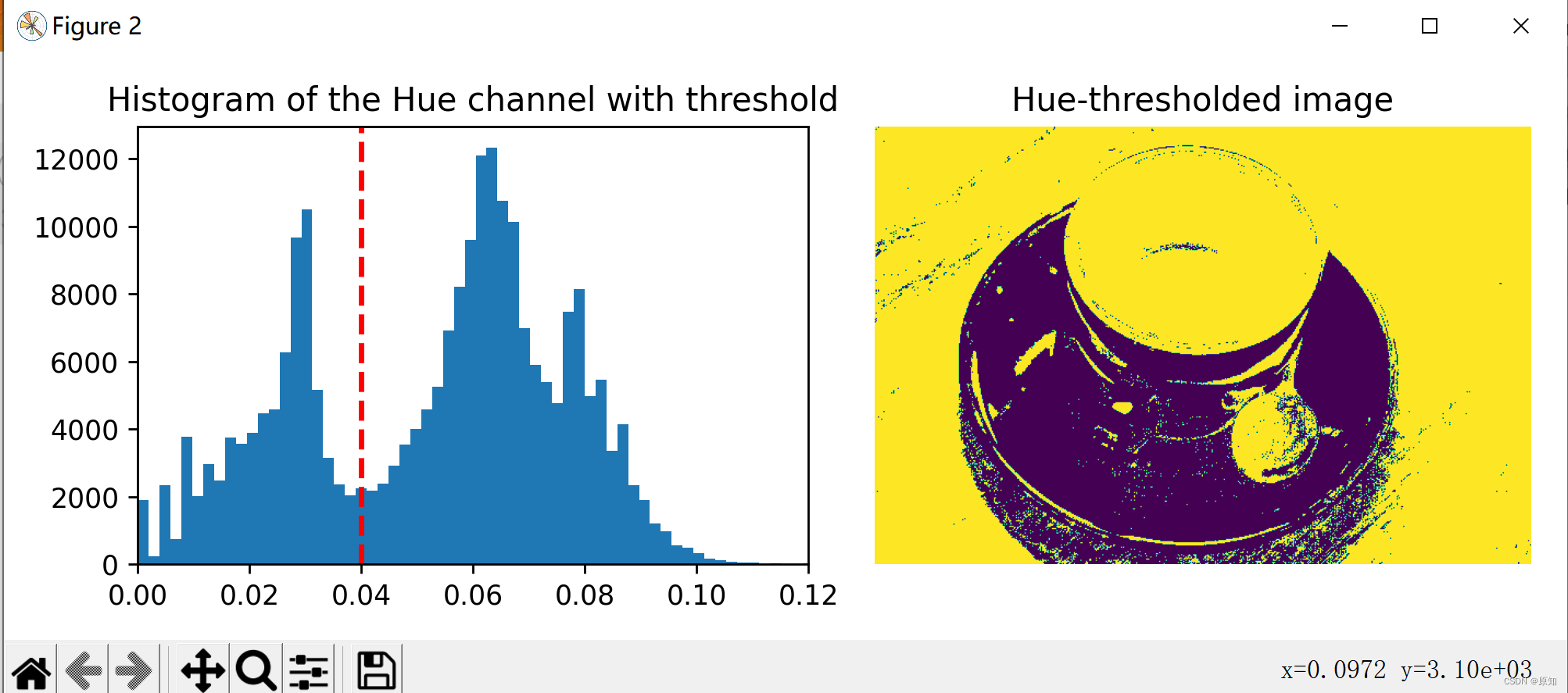
# stay Hue Set a threshold on the channel , Separate the cup from the background :
hue_threshold = 0.04# Why is this passage 0.04
binary_img = hue_img > hue_threshold
fig, (ax0, ax1) = plt.subplots(ncols=2, figsize=(8, 3))
''' plt.hist Function is used to draw histogram . The function prototype : plt.hist(x, bins=None) Parameters x It's a one-dimensional array ,bins It can be understood as the number of rectangles , The default is 10. '''
ax0.hist(hue_img.ravel(), 512)#512 Is the number of histogram bars Set by yourself
ax0.set_title("Histogram of the Hue channel with threshold")#Hue Channel histogram with threshold
#matplotlib Library axiss Module Axes.axvline() The function is used to add a vertical line on the axis .
ax0.axvline(x=hue_threshold, color='r', linestyle='dashed', linewidth=2)
#matplotlib Library axiss Module Axes.set_xbound() Function to set x The upper and lower numerical boundaries of the axis .
ax0.set_xbound(0, 0.12)
ax1.imshow(binary_img)
ax1.set_title("Hue-thresholded image")
ax1.axis('off')
fig.tight_layout()
# stay Value Perform an additional threshold on the channel , Partially remove the shadow of the cup :
fig, ax0 = plt.subplots(figsize=(4, 3))
value_threshold = 0.10
binary_img = (hue_img > hue_threshold) | (value_img < value_threshold)
ax0.imshow(binary_img)
ax0.set_title("Hue and value thresholded image")
ax0.axis('off')
fig.tight_layout()
plt.show()
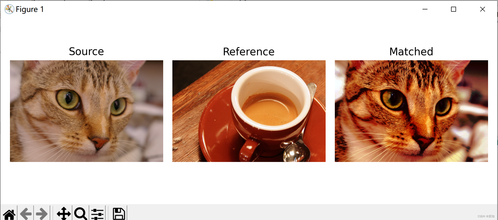
3、 Histogram matching
This example shows the characteristics of histogram matching . It manipulates the pixels of the input image , Match its histogram with the histogram of the reference image .
If the image has more than one channel , As long as the number of channels in the input image and the reference image is equal , Then match each channel independently .
Histogram matching can be used as a lightweight normalization in image processing , For example, feature matching , Especially in images from different sources or different conditions ( Namely light ) In the case of shooting .
import matplotlib.pyplot as plt
from skimage import data
from skimage import exposure
from skimage.exposure import match_histograms
reference = data.coffee()
image = data.chelsea()
matched = match_histograms(image, reference, channel_axis=-1)
''' '''
fig, (ax1, ax2, ax3) = plt.subplots(nrows=1, ncols=3, figsize=(8, 3),
sharex=True, sharey=True)
for aa in (ax1, ax2, ax3):
aa.set_axis_off()
ax1.imshow(image)
ax1.set_title('Source')
ax2.imshow(reference)
ax2.set_title('Reference')
ax3.imshow(matched)
ax3.set_title('Matched')
plt.tight_layout()
plt.show()
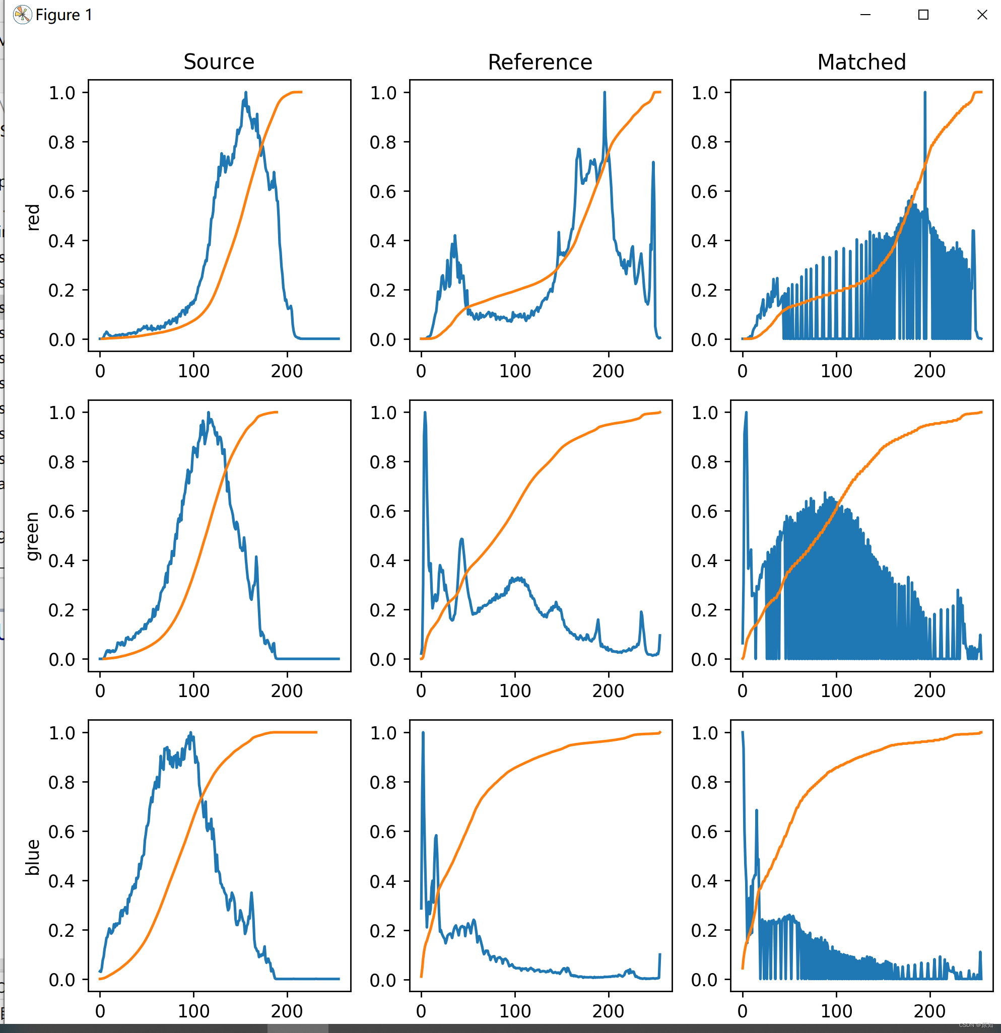
# To illustrate the effect of histogram matching , We draw each RGB Histogram and cumulative histogram of channels .
# Obviously , The matching image of each channel has the same cumulative histogram as the reference image .
fig, axes = plt.subplots(nrows=3, ncols=3, figsize=(8, 8))
#enumerate This adds an index , At the same time, it can read the elements
for i, img in enumerate((image, reference, matched)):
for c, c_color in enumerate(('red', 'green', 'blue')):
img_hist, bins = exposure.histogram(img[..., c], source_range='dtype')
# The largest value of each group of data divided by the data is normalization . The maximum value after processing is 1, Other values are less than 1 Number of numbers .
# In the histogram bin The meaning of : To calculate the color histogram, we need to divide the color space into several small color intervals , That is, histogram bin, The color histogram is obtained by calculating the inner pixels of color in each cell ,bin The more , The stronger the resolution of histogram to color , But it increases the burden of computers . namely ( As shown in the figure above 10 Vertical bar area , Each vertical bar area is called a bin)
axes[c, i].plot(bin, img_hist / img_hist.max())
img_cdf, bins = exposure.cumulative_distribution(img[..., c])
axes[c, i].plot(bins, img_cdf)
axes[c, 0].set_ylabel(c_color)
print(c,i)
axes[0, 0].set_title('Source')
axes[0, 1].set_title('Reference')
axes[0, 2].set_title('Matched')
plt.tight_layout()
plt.show()
annotation :
1、 Returns the histogram of the image
cucim.skimage.exposure.histogram(image, nbins=256, source_range='image', normalize=False)
Returns the histogram of the image , And numpy.histogram Different , This function returns bin Center of , And will not recombine integer arrays .
For integer arrays , Each integer value has its own bin, This improves speed and intensity-resolution.
Calculate histogram on flattened image : For color images , This function should be used separately on each channel to obtain the histogram of each color channel .
Parameters :
image: Array , The input image .
nbins: Integers , Optional , Used to calculate the histogram bin Number . For integer arrays , This value will be ignored .
source_range: character string , Optional ,‘image’( Default ) Determine the range of the input image . ‘dtype’ Determine the expected range of the data type image .
normalize: Boolean type , Optional , If True, The histogram is normalized by the sum of its values .
Return value :
hist: Array , Histogram value .
bin_centers: Array ,bin The value of the center .
2、 Returns the cumulative distribution function of a given image (cdf).
cucim.skimage.exposure.cumulative_distribution(image, nbins=256)
Parameters :
image: Array , Image array .
nbins: Integers , Optional , Image histogram of bin Number .
return :
img_cdf: Array , The value of the cumulative distribution function .
bin_centers: Array , The center of the box .
3、 Histogram matching (histogram matching)
meaning : Make the cumulative histogram of the source image consistent with the target image
from skimage.exposure import match_histograms
Parameters 1: The source image ; Parameters 2: Target image ; Parameters 3: Multi channel matching
matched = match_histograms(image, reference, multichannel=True)
边栏推荐
- Vs2019 configuration matrix library eigen
- LeetCode 403. 青蛙过河 每日一题
- The process of creating custom controls in QT to encapsulating them into toolbars (II): encapsulating custom controls into toolbars
- LeetCode 1155. 掷骰子的N种方法 每日一题
- skimage学习(1)
- LeetCode 1626. 无矛盾的最佳球队 每日一题
- typescript ts基础知识之tsconfig.json配置选项
- LeetCode 1043. 分隔数组以得到最大和 每日一题
- skimage学习(3)——使灰度滤镜适应 RGB 图像、免疫组化染色分离颜色、过滤区域最大值
- AutoLISP series (2): function function 2
猜你喜欢
The latest interview experience of Android manufacturers in 2022, Android view+handler+binder
掌握这个提升路径,面试资料分享
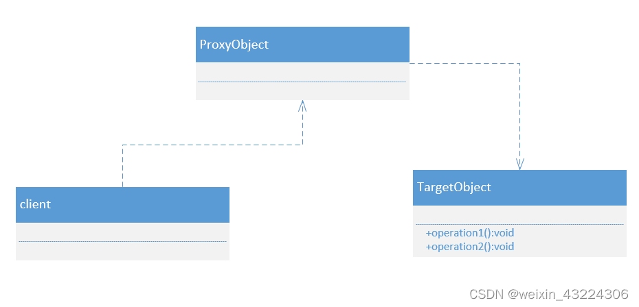
【DesignMode】代理模式(proxy pattern)
skimage学习(2)——RGB转灰度、RGB 转 HSV、直方图匹配
Master this set of refined Android advanced interview questions analysis, oppoandroid interview questions
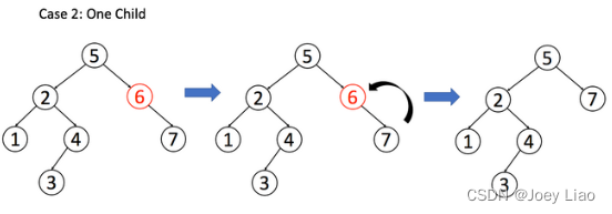
Binary search tree (basic operation)
Personal notes of graphics (3)
数据中台落地实施之法
使用JSON.stringify()去实现深拷贝,要小心哦,可能有巨坑

全网“追杀”钟薛高
随机推荐
《产品经理必读:五种经典的创新思维模型》的读后感
LeetCode 120. 三角形最小路径和 每日一题
水平垂直居中 方法 和兼容
低代码(lowcode)帮助运输公司增强供应链管理的4种方式
【DesignMode】模板方法模式(Template method pattern)
应用在温度检测仪中的温度传感芯片
ByteDance Android gold, silver and four analysis, Android interview question app
typescript ts基础知识之tsconfig.json配置选项
LeetCode 300. Daily question of the longest increasing subsequence
LeetCode 403. Frog crossing the river daily
二叉搜索树(特性篇)
LeetCode 152. Product maximum subarray daily question
The difference and working principle between compiler and interpreter
Opencv personal notes
Vs2019 configuration matrix library eigen
AutoLISP series (3): function function 3
Arduino 控制的双足机器人
ATM系统
SlashData开发者工具榜首等你而定!!!
time标准库