当前位置:网站首页>[secretly kill little partner pytorch20 days] - [Day1] - [example of structured data modeling process]
[secretly kill little partner pytorch20 days] - [Day1] - [example of structured data modeling process]
2022-07-07 02:51:00 【aJupyter】
System tutorial 20 Heaven takes Pytorch
Recently with Brother Zhong 、 Huige Do a little punch in ,20 God pytorch, This is the first day . Welcome to one button and three links .
List of articles
import os
import datetime

# Print time
def printbar():
    nowtime = datetime.datetime.now().strftime('%Y-%m-%d %H:%M:%S')
    print("\n"+"=========="*8 + "%s"%nowtime)

#mac On the system pytorch and matplotlib stay jupyter You need to change the environment variable when running in
os.environ["KMP_DUPLICATE_LIB_OK"]="TRUE"
tips:datetime The module displays the current time and formats 
One 、 Prepare the data
The goal of the Titanic data set is to predict, based on passenger information, whether they will survive the sinking of the Titanic after it hit an iceberg .( You need to focus on the data set and add blog to top the fan group )
Structured data generally uses Pandas Medium DataFrame Pre treatment .
tips: Structured data is simply a database table , Of course csv excel It's all like this
import numpy as np
import pandas as pd
import matplotlib.pyplot as plt
import torch
from torch import nn
from torch.utils.data import Dataset,DataLoader,TensorDataset

dftrain_raw = pd.read_csv('/home/mw/input/data6936/eat_pytorch_data/data/titanic/train.csv')
dftest_raw = pd.read_csv('/home/mw/input/data6936/eat_pytorch_data/data/titanic/test.csv')
dftrain_raw.head(10)

Field description :
Survived:0 For death ,1 For survival 【y label 】
Pclass: The type of ticket held by passengers , There are three values (1,2,3) 【 convert to onehot code 】
Name: Name of passenger 【 Give up 】
Sex: Passenger gender 【 convert to bool features 】
Age: Passenger age ( There is a lack of ) 【 Numerical characteristics , add to “ Is age missing ” As an auxiliary feature 】
SibSp: Passenger brothers and sisters / The number of spouses ( An integer value ) 【 Numerical characteristics 】
Parch: Passenger's parents / The number of children ( An integer value )【 Numerical characteristics 】
Ticket: Ticket number ( character string )【 Give up 】
Fare: The price of a passenger ticket ( Floating point numbers ,0-500 Unequal ) 【 Numerical characteristics 】
Cabin: Passenger cabin ( There is a lack of ) 【 add to “ Is the cabin missing ” As an auxiliary feature 】
Embarked: Passenger boarding port :S、C、Q( There is a lack of )【 convert to onehot code , Four dimensions S,C,Q,nan】
one-hot code ( Hot coding alone ): To put it bluntly, it is to map the data into the corresponding binary
1->001
2->010
3->100
Another example
1: I 2: Love 3: Dad 4: Mom 5: China 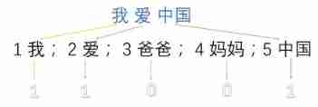
utilize Pandas We can simply carry out the data visualization function of Exploratory data analysis EDA(Exploratory Data Analysis).
label Distribution situation
%matplotlib inline
%config InlineBackend.figure_format = 'png'
ax = dftrain_raw['Survived'].value_counts().plot(kind = 'bar',
     figsize = (12,8),fontsize=15,rot = 0)
ax.set_ylabel('Counts',fontsize = 15)
ax.set_xlabel('Survived',fontsize = 15)
plt.show()

tips:dftrain_raw[‘Survived’].value_counts() The return is series data structure , It can be understood as a one-dimensional dictionary , Students who do not understand this data structure can see Python Advanced —Pandas, There is also a point of attention here series You can go directly through plot How to draw 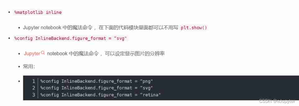
Age distribution
%matplotlib inline
%config InlineBackend.figure_format = 'png'
ax = dftrain_raw['Age'].plot(kind='hist', bins=20, color='purple',
                             figsize=(12, 8), fontsize=15)

ax.set_ylabel('Frequency', fontsize=15)
ax.set_xlabel('Age', fontsize=15)
plt.show()

Age and label The relevance of
%matplotlib inline
%config InlineBackend.figure_format = 'png'
ax = dftrain_raw.query('Survived == 0')['Age'].plot(kind = 'density',
                      figsize = (12,8),fontsize=15)
dftrain_raw.query('Survived == 1')['Age'].plot(kind = 'density',
                      figsize = (12,8),fontsize=15)
ax.legend(['Survived==0','Survived==1'],fontsize = 12)
ax.set_ylabel('Density',fontsize = 15)
ax.set_xlabel('Age',fontsize = 15)
plt.show()
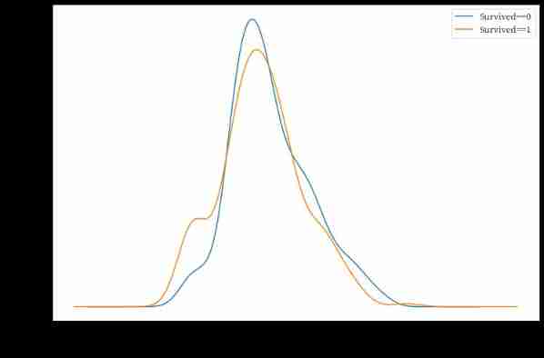
tips: The two curves here use one figure, So the legend and x label 、y Label to bx and ax The settings are the same
dftrain_raw.query(‘Survived == 1’) there query Equivalent to filter conditions
The following is the formal data preprocessing
def preprocessing(dfdata):

    dfresult= pd.DataFrame()

    #Pclass
    dfPclass = pd.get_dummies(dfdata['Pclass'])
    dfPclass.columns = ['Pclass_' +str(x) for x in dfPclass.columns ]
    dfresult = pd.concat([dfresult,dfPclass],axis = 1)

    #Sex
    dfSex = pd.get_dummies(dfdata['Sex'])
    dfresult = pd.concat([dfresult,dfSex],axis = 1)

    #Age
    dfresult['Age'] = dfdata['Age'].fillna(0)
    dfresult['Age_null'] = pd.isna(dfdata['Age']).astype('int32')

    #SibSp,Parch,Fare
    dfresult['SibSp'] = dfdata['SibSp']
    dfresult['Parch'] = dfdata['Parch']
    dfresult['Fare'] = dfdata['Fare']

    #Carbin
    dfresult['Cabin_null'] =  pd.isna(dfdata['Cabin']).astype('int32')

    #Embarked
    dfEmbarked = pd.get_dummies(dfdata['Embarked'],dummy_na=True)
    dfEmbarked.columns = ['Embarked_' + str(x) for x in dfEmbarked.columns]
    dfresult = pd.concat([dfresult,dfEmbarked],axis = 1)

    return(dfresult)

x_train = preprocessing(dftrain_raw).values
y_train = dftrain_raw[['Survived']].values

x_test = preprocessing(dftest_raw).values
y_test = dftest_raw[['Survived']].values

print("x_train.shape =", x_train.shape )
print("x_test.shape =", x_test.shape )

print("y_train.shape =", y_train.shape )
print("y_test.shape =", y_test.shape )

'''  Output : x_train.shape = (712, 15) x_test.shape = (179, 15) y_train.shape = (712, 1) y_test.shape = (179, 1) '''
tips:
pandas Medium get_dummies The method is mainly used to do the classification of category features One-Hot code ( Hot coding alone ).
pd.isna(dfdata[‘Age’]).astype(‘int32’) lookup NaN Value and becomes 1, The rest are not NaN Value to 0
Further use DataLoader and TensorDataset Data can be encapsulated into a pipeline .
dl_train = DataLoader(TensorDataset(torch.tensor(x_train).float(),torch.tensor(y_train).float()),
                     shuffle = True, batch_size = 8)
dl_valid = DataLoader(TensorDataset(torch.tensor(x_test).float(),torch.tensor(y_test).float()),
                     shuffle = False, batch_size = 8)
tips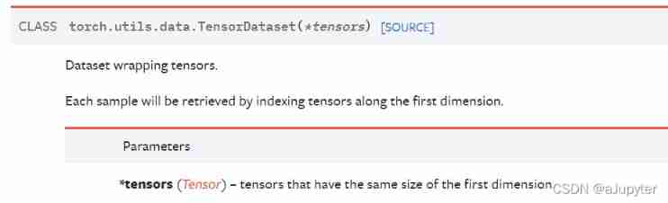
#  Test data pipeline
for features,labels in dl_train:
    print(features,labels)
    break
tensor([[ 0.0000, 0.0000, 1.0000, 0.0000, 1.0000, 0.0000, 1.0000, 0.0000,
0.0000, 7.2292, 1.0000, 1.0000, 0.0000, 0.0000, 0.0000],
[ 0.0000, 0.0000, 1.0000, 0.0000, 1.0000, 26.0000, 0.0000, 1.0000,
0.0000, 7.8542, 1.0000, 0.0000, 0.0000, 1.0000, 0.0000],
[ 1.0000, 0.0000, 0.0000, 0.0000, 1.0000, 28.0000, 0.0000, 1.0000,
0.0000, 82.1708, 1.0000, 1.0000, 0.0000, 0.0000, 0.0000],
[ 0.0000, 0.0000, 1.0000, 0.0000, 1.0000, 26.0000, 0.0000, 2.0000,
0.0000, 8.6625, 1.0000, 0.0000, 0.0000, 1.0000, 0.0000],
[ 0.0000, 0.0000, 1.0000, 1.0000, 0.0000, 9.0000, 0.0000, 4.0000,
2.0000, 31.2750, 1.0000, 0.0000, 0.0000, 1.0000, 0.0000],
[ 0.0000, 0.0000, 1.0000, 0.0000, 1.0000, 0.0000, 1.0000, 0.0000,
0.0000, 14.5000, 1.0000, 0.0000, 0.0000, 1.0000, 0.0000],
[ 0.0000, 0.0000, 1.0000, 0.0000, 1.0000, 0.0000, 1.0000, 0.0000,
0.0000, 7.2292, 1.0000, 1.0000, 0.0000, 0.0000, 0.0000],
[ 0.0000, 1.0000, 0.0000, 0.0000, 1.0000, 19.0000, 0.0000, 0.0000,
0.0000, 10.5000, 1.0000, 0.0000, 0.0000, 1.0000, 0.0000]]) tensor([[1.],
[0.],
[0.],
[0.],
[0.],
[0.],
[0.],
[0.]])
A small summary :
Data processing : The first step is to figure out what each field means , Distinguish what a label is , What are features , Consider which features need to be retained
- For numerical data, keep it
- For category data, it is necessary to carry out independent coding pd.get_dummies()
- For missing data , Except for filling , You also need to add a column to check whether it is a missing value pd.isna() And turn to 0/1
Add :pd.get_dummies(dfdata[‘Embarked’],dummy_na=True)
- dummy_na : bool, default False
Add a column to indicate NaNs, if False NaNs are ignored.
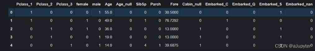
x_train = preprocessing(dftrain_raw)
x_train.head()
Two 、 Defining models
Use Pytorch There are usually three ways to build models :
- Use nn.Sequential Build models in a hierarchical order
- Inherit nn.Module Base classes build custom models
- Inherit nn.Module The base class builds the model and assists in encapsulating the model container .
Here choose the easiest to use nn.Sequential, Hierarchical order model .
def create_net():
    net = nn.Sequential()
    net.add_module("linear1",nn.Linear(15,20))
    net.add_module("relu1",nn.ReLU())
    net.add_module("linear2",nn.Linear(20,15))
    net.add_module("relu2",nn.ReLU())
    net.add_module("linear3",nn.Linear(15,1))
    net.add_module("sigmoid",nn.Sigmoid())
    return net

net = create_net()
print(net)

'''  Output : Sequential( (linear1): Linear(in_features=15, out_features=20, bias=True) (relu1): ReLU() (linear2): Linear(in_features=20, out_features=15, bias=True) (relu2): ReLU() (linear3): Linear(in_features=15, out_features=1, bias=True) (sigmoid): Sigmoid() ) '''
!pip install torchkeras
!pip install prettytable
!pip install datetime


''' Torchkeras Long to see  '''
from torchkeras import summary
summary(net,input_shape=(15,))
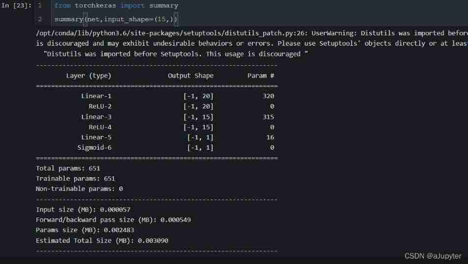
Digression : Isn't that what tensorflow Of summary Function
3、 ... and 、 Training models
Pytorch It usually requires the user to write a custom training cycle , The code style of the training cycle varies from person to person .
Yes 3 Class typical training cycle code style :
- Script form training cycle
- Function form training cycle
- Class form training cycle .
Here is a more general script form .
from sklearn.metrics import accuracy_score

loss_func = nn.BCELoss()
optimizer = torch.optim.Adam(params=net.parameters(),lr = 0.01)
metric_func = lambda y_pred,y_true: accuracy_score(y_true.data.numpy(),y_pred.data.numpy()>0.5)
metric_name = "accuracy"
tips:
accuracy_score Classification accuracy
>>>import numpy as np
>>>from sklearn.metrics import accuracy_score
>>>y_pred = [0, 2, 1, 3]
>>>y_true = [0, 1, 2, 3]
>>>accuracy_score(y_true, y_pred)
0.5
>>>accuracy_score(y_true, y_pred, normalize=False)
2
epochs = 10
log_step_freq = 30

dfhistory = pd.DataFrame(columns = ["epoch","loss",metric_name,"val_loss","val_"+metric_name])
print("Start Training...")
nowtime = datetime.datetime.now().strftime('%Y-%m-%d %H:%M:%S')
print("=========="*8 + "%s"%nowtime)

for epoch in range(1,epochs+1):

    # 1, Training cycle -------------------------------------------------
    net.train()
    loss_sum = 0.0
    metric_sum = 0.0
    step = 1

    for step, (features,labels) in enumerate(dl_train, 1):

        #  Gradient clear
        optimizer.zero_grad()

        #  Forward propagation for loss
        predictions = net(features)
        loss = loss_func(predictions,labels)
        metric = metric_func(predictions,labels)

        #  Back propagation gradient
        loss.backward()
        optimizer.step()

        #  Print batch The level of log
        loss_sum += loss.item()
        metric_sum += metric.item()
        if step%log_step_freq == 0:
            print(("[step = %d] loss: %.3f, "+metric_name+": %.3f") %
                  (step, loss_sum/step, metric_sum/step))

    # 2, Verification cycle -------------------------------------------------
    net.eval()
    val_loss_sum = 0.0
    val_metric_sum = 0.0
    val_step = 1

    for val_step, (features,labels) in enumerate(dl_valid, 1):
        #  Turn off gradient computation
        with torch.no_grad():
            predictions = net(features)
            val_loss = loss_func(predictions,labels)
            val_metric = metric_func(predictions,labels)
        val_loss_sum += val_loss.item()
        val_metric_sum += val_metric.item()

    # 3, Log -------------------------------------------------
    info = (epoch, loss_sum/step, metric_sum/step,
            val_loss_sum/val_step, val_metric_sum/val_step)
    dfhistory.loc[epoch-1] = info

    #  Print epoch The level of log
    print(("\nEPOCH = %d, loss = %.3f,"+ metric_name + \
          " = %.3f, val_loss = %.3f, "+"val_"+ metric_name+" = %.3f")
          %info)
    nowtime = datetime.datetime.now().strftime('%Y-%m-%d %H:%M:%S')
    print("\n"+"=========="*8 + "%s"%nowtime)

print('Finished Training...')


'''  Output : Start Training... ================================================================================2022-02-12 14:58:12 [step = 30] loss: 0.639, accuracy: 0.613 [step = 60] loss: 0.622, accuracy: 0.654 EPOCH = 1, loss = 0.629,accuracy = 0.653, val_loss = 0.551, val_accuracy = 0.714 ================================================================================2022-02-12 14:58:13 [step = 30] loss: 0.559, accuracy: 0.717 [step = 60] loss: 0.557, accuracy: 0.733 EPOCH = 2, loss = 0.555,accuracy = 0.721, val_loss = 0.531, val_accuracy = 0.734 ================================================================================2022-02-12 14:58:13 [step = 30] loss: 0.560, accuracy: 0.746 [step = 60] loss: 0.539, accuracy: 0.756 EPOCH = 3, loss = 0.518,accuracy = 0.768, val_loss = 0.429, val_accuracy = 0.783 ================================================================================2022-02-12 14:58:13 [step = 30] loss: 0.490, accuracy: 0.787 [step = 60] loss: 0.484, accuracy: 0.794 EPOCH = 4, loss = 0.493,accuracy = 0.785, val_loss = 0.513, val_accuracy = 0.741 ================================================================================2022-02-12 14:58:13 [step = 30] loss: 0.518, accuracy: 0.779 [step = 60] loss: 0.470, accuracy: 0.806 EPOCH = 5, loss = 0.476,accuracy = 0.799, val_loss = 0.460, val_accuracy = 0.799 ================================================================================2022-02-12 14:58:13 [step = 30] loss: 0.526, accuracy: 0.758 [step = 60] loss: 0.477, accuracy: 0.800 EPOCH = 6, loss = 0.465,accuracy = 0.803, val_loss = 0.482, val_accuracy = 0.793 ================================================================================2022-02-12 14:58:13 [step = 30] loss: 0.520, accuracy: 0.775 [step = 60] loss: 0.470, accuracy: 0.798 EPOCH = 7, loss = 0.468,accuracy = 0.795, val_loss = 0.469, val_accuracy = 0.772 ================================================================================2022-02-12 14:58:13 [step = 30] loss: 0.459, accuracy: 0.825 [step = 60] loss: 0.474, accuracy: 0.810 EPOCH = 8, loss = 0.481,accuracy = 0.794, val_loss = 0.452, val_accuracy = 0.783 ================================================================================2022-02-12 14:58:13 [step = 30] loss: 0.496, accuracy: 0.767 [step = 60] loss: 0.474, accuracy: 0.779 EPOCH = 9, loss = 0.474,accuracy = 0.787, val_loss = 0.443, val_accuracy = 0.793 ================================================================================2022-02-12 14:58:13 [step = 30] loss: 0.424, accuracy: 0.838 [step = 60] loss: 0.481, accuracy: 0.804 EPOCH = 10, loss = 0.478,accuracy = 0.787, val_loss = 0.423, val_accuracy = 0.799 ================================================================================2022-02-12 14:58:13 Finished Training... '''
tips: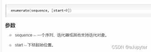
Four 、 Evaluation model
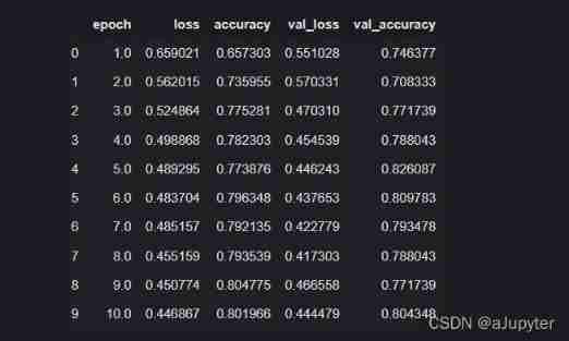
Let's first evaluate the effect of the model on the training set and validation set .
dfhistory
%matplotlib inline
%config InlineBackend.figure_format = 'svg'
import matplotlib.pyplot as plt
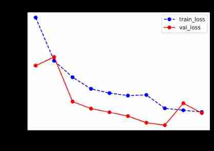
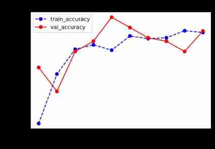
def plot_metric(dfhistory, metric):
train_metrics = dfhistory[metric]
val_metrics = dfhistory['val_'+metric]
epochs = range(1, len(train_metrics) + 1)
plt.plot(epochs, train_metrics, 'bo--')
plt.plot(epochs, val_metrics, 'ro-')
plt.title('Training and validation '+ metric)
plt.xlabel("Epochs")
plt.ylabel(metric)
plt.legend(["train_"+metric, 'val_'+metric])
plt.show()
plot_metric(dfhistory,"loss")
plot_metric(dfhistory,"accuracy")
5、 ... and 、 Using the model
# Prediction probability
y_pred_probs = net(torch.tensor(x_test[0:10]).float()).data
y_pred_probs
''' tensor([[0.1430], [0.6967], [0.3841], [0.6717], [0.6588], [0.9006], [0.2218], [0.8791], [0.5890], [0.1544]]) '''
```python
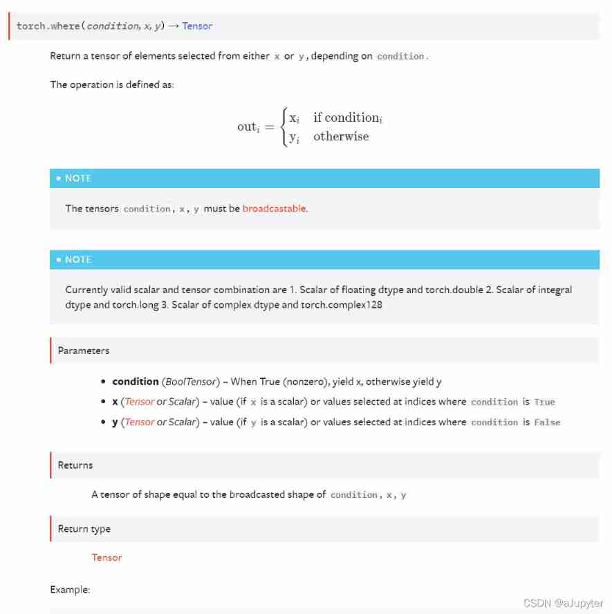
# Forecast category
y_pred = torch.where(y_pred_probs>0.5,
torch.ones_like(y_pred_probs),torch.zeros_like(y_pred_probs))
y_pred
''' tensor([[0.], [1.], [0.], [1.], [1.], [1.], [0.], [1.], [1.], [0.]]) '''
**tips:**
```python
torch.tensor(1).numpy() # array(1)
torch.tensor(1).data # tensor(1)
torch.tensor(1).item() # 1  Use only for scalars
torch.tensor(1).float() #  Convert to floating point  tensor(1.)
torch.tensor(1).int() #  Turn into int32 tensor(1, dtype=torch.int32)
6、 ... and 、 Save the model
Pytorch There are two ways to save models , All by calling pickle The serialization method implements .
The first method only saves model parameters .
The second way to save the entire model .
The first one is recommended , The second method may cause various problems when switching devices and directories .
1, Save model parameters ( recommend )
print(net.state_dict().keys())

''' odict_keys(['linear1.weight', 'linear1.bias', 'linear2.weight', 'linear2.bias', 'linear3.weight', 'linear3.bias']) '''
#  Save model parameters

torch.save(net.state_dict(), "./data/net_parameter.pkl")

net_clone = create_net()
net_clone.load_state_dict(torch.load("./data/net_parameter.pkl"))

net_clone.forward(torch.tensor(x_test[0:10]).float()).data

''' tensor([[0.1327], [0.8162], [0.4354], [0.5858], [0.6404], [0.9614], [0.1819], [0.8931], [0.5858], [0.2205]]) '''
2, Save the complete model ( Not recommended )
torch.save(net, './data/net_model.pkl')
net_loaded = torch.load('./data/net_model.pkl')
net_loaded(torch.tensor(x_test[0:10]).float()).data

''' tensor([[0.0119], [0.6029], [0.2970], [0.5717], [0.5034], [0.8655], [0.0572], [0.9182], [0.5038], [0.1739]]) '''
边栏推荐
- 安全交付工程师
- 数字滚动增加效果
- Matlb| economic scheduling with energy storage, opportunity constraints and robust optimization
- Code line breaking problem of untiy text box
- Redis introduction complete tutorial: client case analysis
- MATLB|具有储能的经济调度及机会约束和鲁棒优化
- Number theory --- fast power, fast power inverse element
- Pioneer of Web3: virtual human
- Wireshark installation
- Google Earth Engine(GEE)——Landsat 全球土地调查 1975年数据集
猜你喜欢


随机推荐
Derivative, partial derivative, directional derivative
【Node学习笔记】chokidar模块实现文件监听
导数、偏导数、方向导数
Redis入门完整教程:AOF持久化
[Mori city] random talk on GIS data (II)
What management points should be paid attention to when implementing MES management system
MySQL提升大量数据查询效率的优化神器
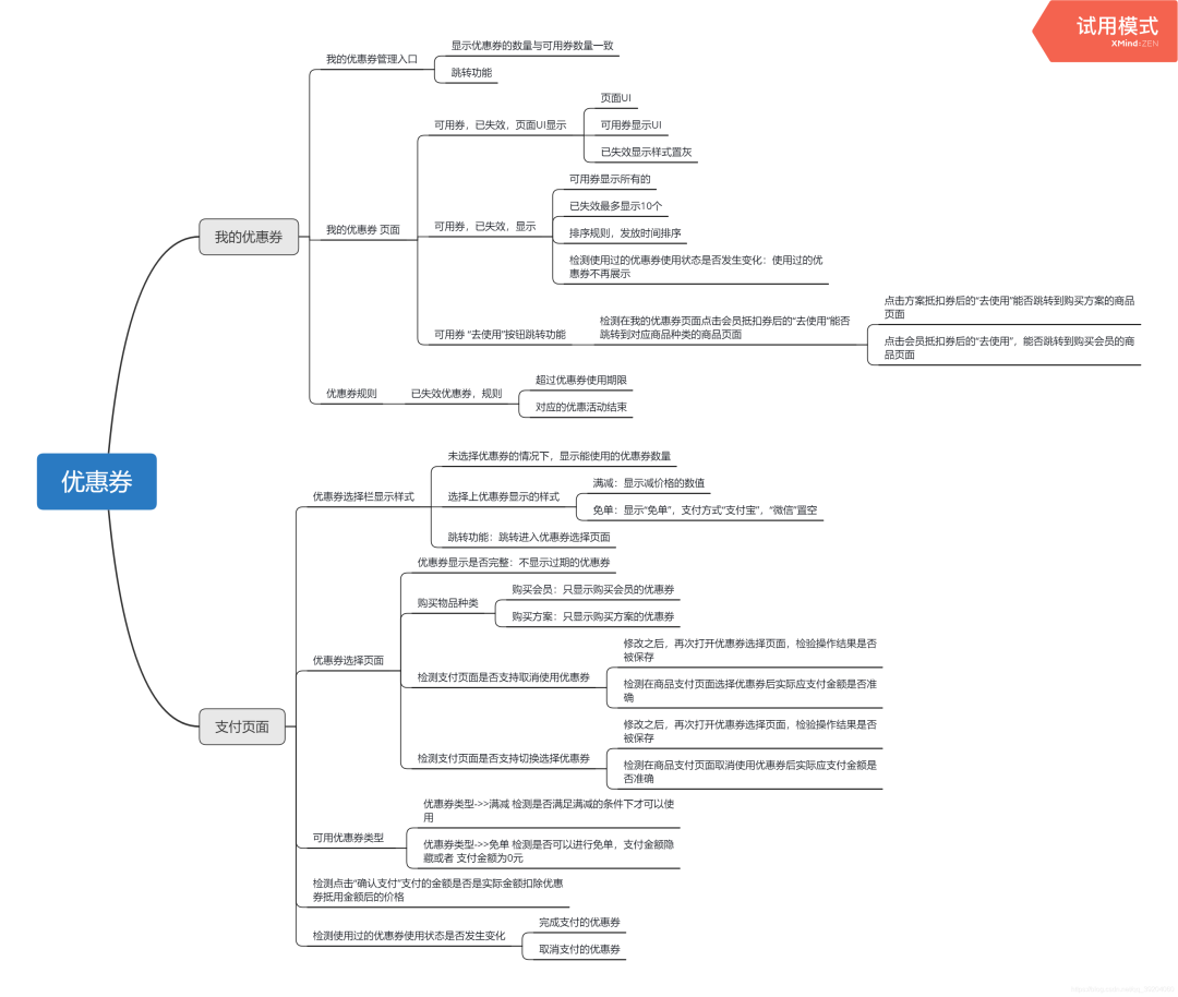
How to write test cases for test coupons?
差异与阵列和阵列结构和链表的区别
Leetcode:minimum_depth_of_binary_tree解决问题的方法
MMDetection3D加载毫米波雷达数据
服装企业部署MES管理系统的五个原因
Read fast RCNN in one article
MySQL
C language exercises_ one
Cloud Mail .NET Edition
普通测试年薪15w,测试开发年薪30w+,二者差距在哪?
【软件测试】最全面试问题和回答,全文背熟不拿下offer算我输
Statistics of radar data in nuscenes data set
QT common Concepts-1