This paper proposes a more general feature-related noise category PMD, Based on this kind of noise, a data calibration strategy is constructed PLC To help the model converge better , Experiments on generated datasets and real datasets have proved the effectiveness of the algorithm . The scheme theory proposed in this paper is proved to be complete , It is very simple to apply , It's worth trying
source : Xiaofei's algorithm Engineering Notes official account
The paper : Learning with Feature-Dependent Label Noise: A Progressive Approach
- Address of thesis :https://arxiv.org/abs/2103.07756v3
- Paper code :https://github.com/pxiangwu/PLC
Introduction
In large datasets , Due to the ambiguity of the label and the carelessness of the annotator , Wrong annotation is inevitable . Because noise has a great impact on supervised training , So it is very important to study how to deal with wrong annotation in practical application .
Some classical methods carry out independent and identically distributed noise (i.i.d.) Assumptions , It is considered that noise has nothing to do with data characteristics , It has its own rules . These methods either directly predict the noise distribution to distinguish the noise , Or introduce additional regular terms / Loss term to distinguish noise . Other methods prove , The commonly used loss term itself can resist these independent and identically distributed noises , Don't care .
Although these methods have theoretical guarantee , But in reality, the performance is poor , Because the assumption of independent and identically distributed noise is not true . It means , The noise of the data set is diverse , And it is related to data characteristics , For example, a fuzzy cat may be mistaken for a dog . In case of insufficient light or blocking , The picture has lost important visual discrimination clues , It is easy to be mislabeled . In order to meet this real challenge , Dealing with noise requires not only effective , Its versatility is also very necessary .
SOTA Most methods use data recalibration (data-recalibrating) Strategies to adapt to a variety of data noise , This strategy gradually confirms the trusted data or gradually corrects the label , Then use these data for training . As data sets become more accurate , The accuracy of the model will gradually improve , Finally, it converges to high accuracy . This strategy makes good use of the learning ability of deep network , Get good results in practice .
But at present, there is no complete theoretical proof of the internal mechanism of these strategies , Explain why these strategies can make the model converge to the ideal state . This means that these strategies are case by case Of , Super parameters need to be adjusted very carefully , Difficult to be universal .
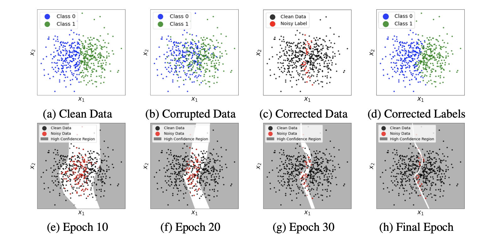
Based on the above analysis , The paper defines the more common PMD Noise family (Polynomial Margin Dimishing Noise Family), Contains any type of noise except obvious errors , More in line with the real scene . be based on PMD Noise family , This paper proposes a data calibration method with theoretical guarantee , The labels of the data are calibrated step by step according to the confidence of the noise classifier . Flow chart 1 Shown , Start with high confidence data , Use the prediction results of the noise classifier to calibrate these data , Then use the calibrated data to improve the model , Carry out label calibration and model upgrading alternately until the model converges .
Method
First define some mathematical symbols , Take the two category task as an example :
- Define feature space \(\mathcal{X}\), data \((x,y)\) From the distribution \(D=\mathcal{X}\times\{0,1\}\) From sampling .
- Definition \(\eta(x)=\mathbb{P}[y=1|x]\) It's a posterior probability , The higher the value, the more obvious the positive label is , The smaller the value, the more obvious the negative label .
- Define the noise function \(\tau_{0,1}(x)=\mathbb{P}=[\tilde{y}=1 | y=0, x]\) and \(\tau_{1,0}(x)=\mathbb{P}=[\tilde{y}=0 | y=1, x]\), among \(\tilde{y}\) Label for errors . Hypothetical data \(x\) The real label is \(y=0\), Then there are \(\tau_{0,1}(x)\) Probability is incorrectly labeled 1.
- Definition \(\tilde{\eta}(x)=\mathbb{P}[\tilde{y}=1|x]\) Is the posterior probability of noise .
- Definition \(\eta^{*}(x)=\mathbb{I}_{\eta(x)\ge\frac{1}{2}}\) Bayesian optimal classifier , When A To true \(\mathbb{I}_A=1\), Otherwise 0.
- Definition \(f(x):\mathcal{X}\to [0,1]\) Scoring function for classifier , It's usually online softmax Output .
Poly-Margin Diminishing Noise
PMD Noise is only a function of noise \(\tau\) Bound to a specific \(\eta(x)\) Middle zone , Noise function in the region \(\tau\) It doesn't matter how much it's worth . This form can not only cover feature independent scenes , It can also be generalized to some specific scenes of previous noise research .

PMD The definition of noise is shown above ,\(t_0\) It can be considered as the space between the left and right (margin).PMD Conditions only require \(\tau\) The upper bound of is polynomial and monotonically decreases in the confidence region of Bayesian classifier , and \(\tau_{0,1}(x)\) and \(\tau_{1,0}(x)\) stay \(\{ x:|\eta(x)-\frac{1}{2}| < t_0 \}\) Any value in the area .
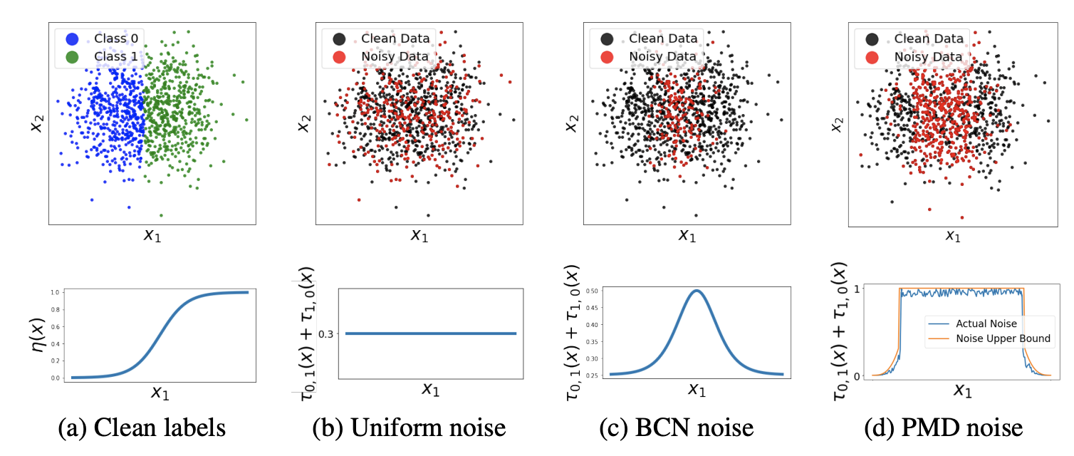
Ahead PMD Noise description may be abstract , The paper provides visual pictures to help you understand :
- chart a It is the result of Bayesian optimal classifier , That is, the correct label . From below \(\eta(x)\) The curve shows , The binary classification probability of the data on both sides is quite different , It is easy to distinguish . The binary classification probability of the intermediate data is relatively close , There is a great possibility of mismarking , That's what we need to focus on .
- chart b It's uniform noise , The noise considers that the misclassification probability is independent of the characteristics , Every data point has the same probability of being misclassified . The black in the above figure is the data that is considered to be correct , Red is the data considered as noise , You can see , After uniform noise treatment , The data distribution is chaotic .
- chart c yes BCN noise , The noise value increases with \(\eta^{*}(x)\) The confidence of . As can be seen from the above figure , The processed noise data basically fall in the middle area , That is, where it is easy to be mistaken . But because of BCN The boundary of noise and \(\eta^{*}(x)\) Highly correlated , In practice, we usually use the output of the model to approximate \(\eta^{*}(x)\), Obviously, there will be a big difference in the scene with a high degree of noise .
- chart d yes PMD noise , Constrain the noise in \(\eta^{*}(x)\) In the middle of , The noise value in the area is arbitrary . The advantage of doing so is , Different noise levels can be dealt with by adjusting the size of the area , As long as it's not an obvious mistake ( That is to say \(\eta\) The higher and lower parts are marked incorrectly ) apply . As can be seen from the above figure , The processed clean data is basically distributed on both sides , That is, where I believe .
The Progressive Correction Algorithm
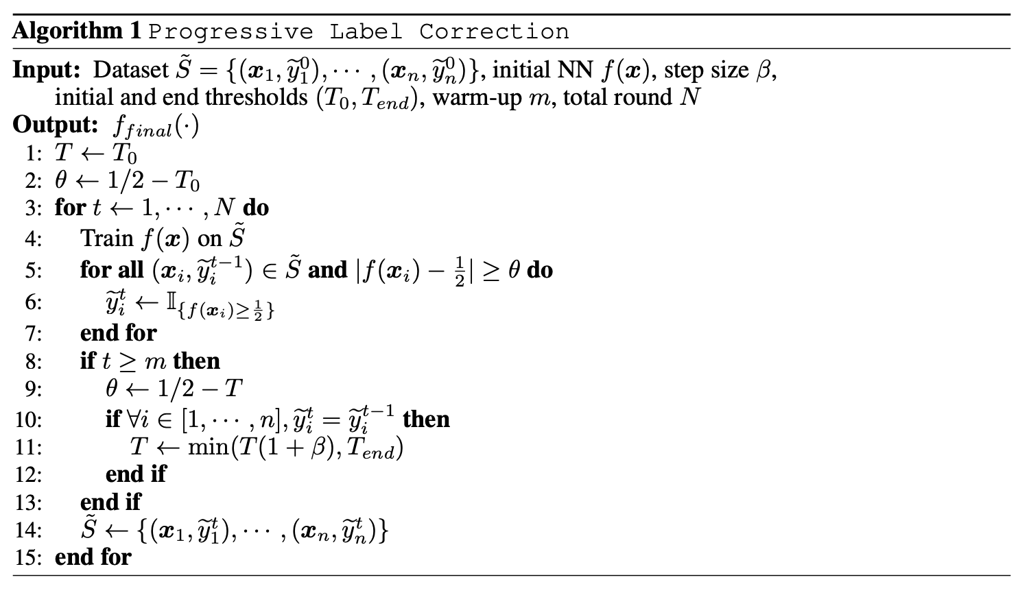
be based on PMD noise , The paper proposes to train and correct labels step by step PLC(Progressive Label Correction) Algorithm . The algorithm first uses the original data set warm-up Stage training , Get a preliminary network that has not been fitted with noise . next , Use warm-up The preliminary network obtained corrects the labels of high confidence data , The paper holds that ( The theory also proves ) Noise classifier \(f\) High confidence prediction can be compared with Bayesian optimal classifier \(\eta^{*}\) bring into correspondence with .
When correcting labels , First select a high threshold \(\theta\). If \(f\) Forecast label and label \(\tilde{y}\) Different and the prediction confidence is higher than the threshold , namely \(|f(x)-1/2|>\theta\), Will \(\tilde{y}\) Corrected to \(f\) The forecast tab . Repeat the label correction and retrain the model with the corrected data set , Until no labels are corrected .
next , Lower the threshold slightly \(\theta\), Repeat the above steps with the reduced threshold , Until the model converges . In order to facilitate the later theoretical analysis , This paper defines a continuously increasing threshold \(T\), Give Way \(\theta=1/2-T\), Specific logic such as Algorithm 1 Shown .
Generalizing to the multi-class scenario
The above descriptions are all binary scenes , In a multi category scenario , First define \(f_i(x)\) Label for classifier \(i\) The probability of prediction ,\(h_x=argmax_if_i(x)\) Tags predicted for the classifier . take \(|f(x)-\frac{1}{2}|\) The judgment of is modified as |\(f_{h_x}(x)-f_{\tilde{y}}(x)|\), When the result is greater than the threshold \(\theta\) when , Label \(\tilde{y}\) Change to label \(h_x\). In the process of practice , Adding logarithm to the difference judgment will be more robust .
Analysis
This is the core of the paper , Mainly from the theoretical point of view to verify the universality and correctness of the proposed method . We won't go on here , If you are interested, please go to the original , We only need to know the usage of this algorithm .
Experiment
At present, there is no public data set for the noise problem of data sets , So we need to generate data sets for experiments , This paper is mainly about CIFAR-10 and CIFAR-100 Data generation and experiment on . First train a network on the original data , The prediction probability of the network is used to approximate the real posterior probability \(\eta\). be based on \(\eta\) Resample data \(x\) The label of \(y_x\sim\eta(x)\) As a clean data set , The previously trained network is used as the Bayesian optimal classifier \(\eta^{*}:\mathcal{X}\to\{1,\cdots,C\}\), among \(C\) Is the number of categories . It should be noted that , In multi category scenarios ,\(\eta(x)\) Output as vector ,\(\eta_i(x)\) The number of the corresponding vector \(i\) Elements .
For the generation of noise , There are characteristic correlation noise and independent identically distributed noise (i.d.d) Two kinds of :
- For feature related noise , In order to increase the challenge of noise , Every data \(x\) According to the noise function, it is possible to classify from the highest confidence \(u_x\) Become the second confidence classification \(s_x\), Where the noise function and \(\eta(x)\) Probability Correlation .\(s_x\) about \(\eta^{*}(x)\) It is the category with the highest degree of confusion , It can most affect the performance of the model . in addition , because \(y_x\) It's from \(\eta(x)\) From sampling , It is the category with the highest confidence , So it can be considered that \(y_x\) Namely \(u_x\). Overall speaking , For data \(x\), When generating data, it either becomes \(s_x\), Or keep \(u_x\). There are three kinds of feature related noise PMD Noise function in noise family :

because \(\eta(x)\) It can't be modified , In order to control the noise level , The only thing that can be done is for the noise function \(\tau_{u_x,s_x}\) Add a constant factor , Make the final noise ratio meet the expectations . about PMD noise ,35% and 70% The noise level of represents 35% and 70% The clean data of is modified into noise . - Independent identically distributed noise by constructing noise transformation matrix \(T\) To modify the label , among \(T_{ij}=P(\tilde{y}=j|y=i)=\tau_{ij}\) For real labels \(y=i\) Convert to label \(j\) Probability . For the label \(i\) The data of , Change its label to from matrix \(T\) Of the \(i\) Labels sampled from the probability distribution of rows . This paper adopts two kinds of common independent identically distributed noise :1) Uniform noise (Uniform noise), Real label \(i\) The probability of converting to other tags is the same , namely \(T_{ij}=\tau/(C-1)\), among \(i\ne j\),\(T_{ii}=1-\tau\),\(\tau\) Is the noise level .2) Asymmetric noise (Asymmetric noise), Real label \(i\) There is a probability \(T_{ij}=\tau\) Probability is converted into labels \(j\), or \(T_{ii}=1-\tau\) The probability remains the same .
In the experiment , Some experiments will combine feature related noise and independent identically distributed noise to generate and experiment noise data sets , The final verification standard is the accuracy of the model on the verification set . During training , use 128 batch size、0.01 Learning rate and SGD Optimizer , Co training 180 Period guarantees convergence , repeat 3 Take the mean and standard deviation for the second time .
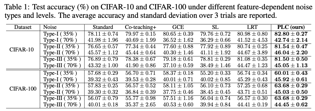
PMD Noise test , stay 35% and 70% Performance comparison under noise level .
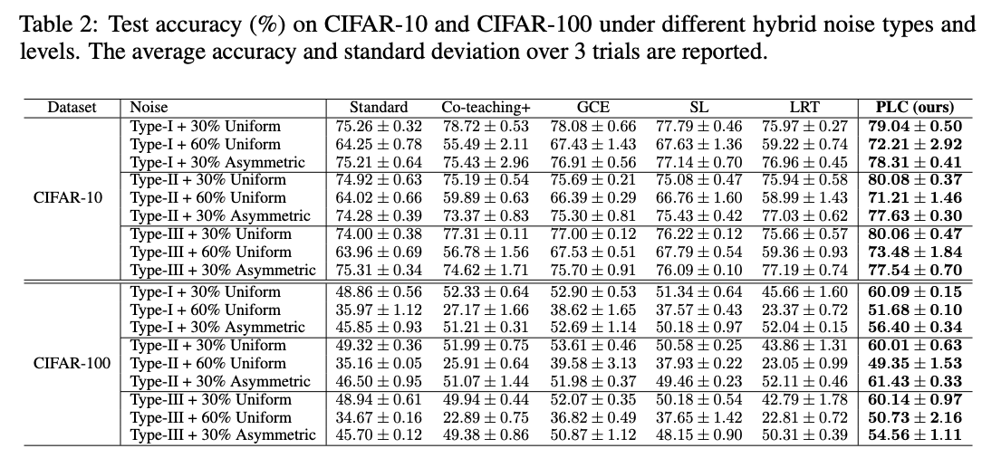
Mixed noise test , stay 50%-70% Performance comparison under noise level .

Superparametric comparative experiment .

Performance comparison on real data sets .
Conclusion
This paper proposes a more general feature-related noise category PMD, Based on this kind of noise, a data calibration strategy is constructed PLC To help the model converge better , Experiments on generated datasets and real datasets have proved the effectiveness of the algorithm . The scheme theory proposed in this paper is proved to be complete , It is very simple to apply , It's worth trying .
If this article helps you , Please give me a compliment or watch it ~
More on this WeChat official account 【 Xiaofei's algorithm Engineering Notes 】

