当前位置:网站首页>Introduction and case analysis of Prophet model
Introduction and case analysis of Prophet model
2022-07-06 18:16:00 【Know the cold and the warm*】
Catalog
- Preface
- One 、Prophet Installation and introduction
- Two 、 Applicable scenario
- 3、 ... and 、 Input and output of the algorithm
- Four 、 Algorithm principle
- 5、 ... and 、 Parameters that can be set when using
- 6、 ... and 、 Learning materials reference
- 7、 ... and 、 Model application
- 7-1、 Stock price forecast
- 7-2、 Battery Diviner
- 7-2-1、 Import related libraries
- 7-2-2、 Reading data
- 7-2-3、 Data preprocessing and the division of training set and test set .
- 7-2-4、 Instantiation Prophet object , And through fit To train the model
- 7-2-5、 Data visualization
- 7-2-6、 Compare the predicted value with the real value
- 7-2-7、 Model to evaluate
- 7-2-7、 Model storage
- 8、 ... and 、 Other matters needing attention
- summary
Preface
prophet yes facebook An open source time series prediction algorithm .
One 、Prophet Installation and introduction
1、 brief introduction : Time series prediction algorithm Prophet yes Facebook The team open source a time series prediction algorithm , The algorithm combines time series decomposition and machine learning algorithm , And it can predict the time series with missing values and outliers .
2、 install :
Use conda command :( If not installed anaconda Please check out my other article :Anaconda And some common operations .)
conda install pystan
conda install -c conda-forge prophet
Two 、 Applicable scenario
Applicable to those with obvious internal laws 、 Periodic data , For example, seasonal changes , Holiday trend .
3、 ... and 、 Input and output of the algorithm
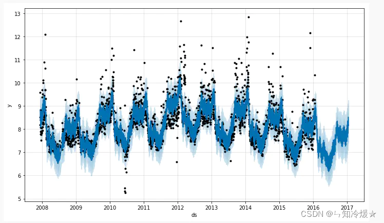
Black dots : Represents the discrete points of the original time series
Dark blue line : Represents the value obtained by fitting with time series
Light blue line : Represents a confidence interval of the time series , That is, the so-called reasonable upper and lower bounds
Prophet Input and output of the model : Enter the timestamp of the known time series and the corresponding value ; Enter the length of the time series to be predicted ; Output the trend of future time series . The output results can provide the necessary statistical indicators , Including fitting curve , Upper and lower bounds, etc .
Pass in prophet The data of : Divided into two columns ,ds and y,ds Represents the timestamp of the time series ( yes pandas Date format for ),y Represents the value of the time series ( Numerical data ),Prophet Default fields for , Must be named ds and y These two columns . In general ,y To normalize
df['y'] = (df['y'] - df['y'].mean()) / (df['y'].std())
prophet The predicted value of the output :yhat, Represents the predicted value of the time series ;yhat_lower, Represents the lower bound of the predicted value ;yhat_upper, Represents the upper bound of the predicted value .
Four 、 Algorithm principle
1、 principle : Because in reality , Time series are often composed of trend items , Season item , The holiday effect is composed of emergencies and residual items , therefore Prophet The algorithm adopts the method of time series decomposition , It divides the time series into these parts :
y ( t ) = g ( t ) + s ( t ) + h ( t ) + α y(t)=g(t)+s(t)+h(t)+α y(t)=g(t)+s(t)+h(t)+α
Among them g ( t ) g(t) g(t) Represents a trend item , It reflects the non periodic change trend of time series ; s ( t ) s(t) s(t) Indicates seasonal items , It reflects the periodic changes of time series , Like every week , This seasonal change every year ; h ( t ) h(t) h(t) Represents a holiday item , It reflects the irregular changes that last from one day to several days, such as holidays ; final α α α Represents the residual term , Usually normally distributed . Then each item is fitted separately , The final cumulative result is Prophet The prediction results of the algorithm .
2、 advantage :
(1)、 The measured data does not need regular intervals .
(2)、 We don't need to insert missing values or delete outliers , namely Prophet Be friendly to missing values , Sensitive to outliers .
(3)、 The parameters of the prediction model are easy to explain .
3、 Other tuning strategies
(1)、 By default, the model grows according to the linear trend , But if you follow log Mode growth , Can be adjusted growth = ‘logistic’, Logistic regression model .
(2)、 When we know in advance that one day will affect the overall trend of the data , You can set this day as a turning point .
(3)、 For holidays , Can pass holday To adjust , For different holidays , You can adjust different front and back window periods . for example : Spring Festival has 7 Japan , But the impact of Spring Festival travel is approaching 30 Japan .
5、 ... and 、 Parameters that can be set when using
Prophet Default parameters :
def __init__(
    self,
    growth='linear',
    changepoints=None,
    n_changepoints=25,
    changepoint_range=0.8,
    yearly_seasonality='auto',
    weekly_seasonality='auto',
    daily_seasonality='auto',
    holidays=None,
    seasonality_mode='additive',
    seasonality_prior_scale=10.0,
    holidays_prior_scale=10.0,
    changepoint_prior_scale=0.05,
    mcmc_samples=0,
    interval_width=0.80,
    uncertainty_samples=1000,
):
1、growth: Growth trend model , It is divided into “linear” And “logistic”, Represent linear and nonlinear growth respectively , The default value is linear.
2、Capacity: When the increment function is a logistic regression function , The capacity value to be set , Indicates the maximum value defined in the nonlinear growth trend , The predicted value will reach saturation at this point .
3、Change Points: Can pass n_changepoints and changepoint_range To set equidistant change points , The change point of time series can also be specified by manual setting , The default value is :“None”.
4、n_changepoints: User specified potential ”changepoint” The number of , The default value is :25.
5、changepoint_prior_scale: The flexibility of the growth trend model . Adjust the ”changepoint” Flexibility of choice , The bigger the value is. , Select the ”changepoint” The more , Thus, the fitting degree of the model to the historical data becomes stronger , However, it also increases the risk of over fitting . The default value is :0.05.
6、seasonality_prior_scale(seasonality In the model ): Adjust the intensity of seasonal components . The bigger the value is. , The model will adapt to stronger seasonal fluctuations , The smaller the value. , The more seasonal fluctuations are suppressed , The default value is :10.0.
7、holidays_prior_scale(holidays In the model ): Adjust the strength of the model components . The bigger the value is. , The greater the impact of the holiday on the model , The smaller the value. , The smaller the impact of holidays , The default value is :10.0.
8、freq: The statistical unit of time in data ( frequency ), The default is ”D”, Count by day .
9、periods: The number of future times to be predicted . For example, statistics by day , Want to predict what will happen in the next year , You need to fill in 365.
10、mcmc_samples:mcmc sampling , Used to get the uncertainty of predicting the future . If more than 0, Will do mcmc Full Bayesian inference of samples , If 0, We will do the maximum a posteriori estimation , The default value is :0.
11、interval_width: Measure the extent to which trends change in the future . Indicates the similarity between the frequency and amplitude of trend intervals used in future prediction and historical data , The larger the value, the more similar , The default value is :0.80. When mcmc_samples = 0 when , This parameter is only used for the change degree of the growth trend model , When mcmc_samples > 0 when , It also includes the degree of seasonal change .
12、uncertainty_samples: The number of simulation plots used to estimate the growth trend interval in the future , The default value is :1000.
13、yearly_seasonality: Is the data seasonal , Default “ Automatic detection ”.
14、weekly_seasonality: Whether the data has weekly seasonality , Default “ Automatic detection ”.
15、daily_seasonality: Whether the data is seasonal , Default “ Automatic detection ”.
16、seasonality_mode: Seasonal effect pattern , Default addition mode “additive”, Optional “multiplicative” Multiplication mode .
6、 ... and 、 Learning materials reference
7、 ... and 、 Model application
7-1、 Stock price forecast
7-1-1、 Import related libraries
from prophet import Prophet
import numpy as np
import matplotlib.pyplot as plt
import pandas as pd
7-1-2、 Reading data
#  Reading data
df = pd.read_csv('./018/000001_Daily_2006_2017.csv')
#  Select the date and closing price
df = df[['date','Close']]
data : We only need the date and closing price , namely date and Close These two columns .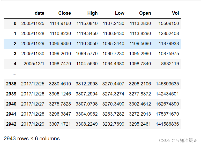
7-1-3、 Data preprocessing and the division of training set and test set .
#  Be careful :Prophet The model has requirements for data format , The date field must be datetime Format , Through here pd.to_datetime To switch .
df['date'] = pd.to_datetime(df['date'])
#  Here we need to adjust the closing price log Handle , It can be understood as normalization , Note that the closing price needs to be restored when the final drawing .
df['Close'] = np.log(df['Close'])
#  Change column name , Change to Prophet Specified column name ds and y
df = df.rename(columns={
    'date': 'ds', 'Close': 'y'})
#  Divide the data , It is divided into training set and verification set , Take the data of the previous ten years as the training set , The data of the next year is used as the test set .
df_train = df[:2699]
df_test = df[2699:]
current df As shown in the figure :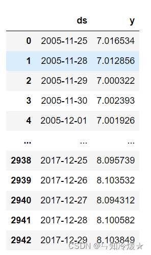
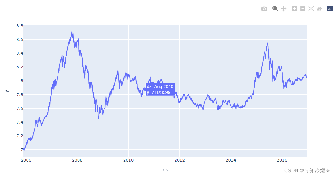
Observation data : Observe historical data , See a little trend .
import plotly.express as px

fig = px.line(df_train, x="ds", y="y")
fig.show()
7-1-4、 Instantiation Prophet object , And through fit To train the model
model = Prophet()
model.fit(df_train)
# make_future_dataframe:  The function is to tell the model how long we want to predict , And what is the period of time . I'm going to set it to 365, That is, the data that predicts a year .
# future = model.make_future_dataframe(periods=365, freq='D')
#  To make predictions , Return the predicted result forecast
forecast = model.predict(future)
# forecast['additive_terms'] = forecast['weekly'] + forecast['yearly'];
#  Yes :forecast['yhat']  = forecast['trend'] +  forecast['additive_terms'] .
#  therefore :forecast['yhat']  = forecast['trend'] +forecast['weekly'] + forecast['yearly'].
#  If there are holidays , Then there will be forecast['yhat']  = forecast['trend'] +forecast['weekly'] + forecast['yearly'] + forecast['holidays'].
forecast
forecast Express :Dataframe It contains a lot of information about the predicted results , among yhat Indicates the predicted result .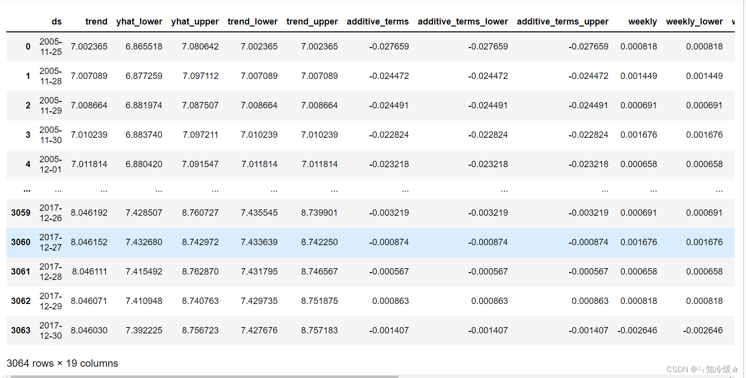
7-1-5、 Data visualization
# Visual operation of data models , Black dots represent real data , The blue line indicates the prediction result . The blue area indicates the upper and lower prediction limits under a certain degree of confidence .
model.plot(forecast)
plt.show()
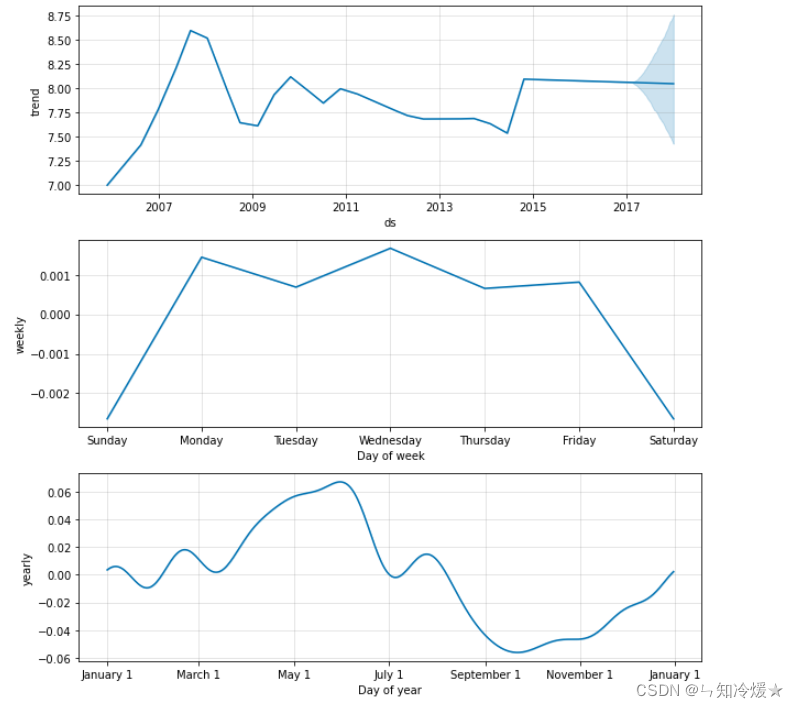
# adopt plot_componets() It can realize the year of data 、 month 、 Visualization of trends in different time periods of the week .
model.plot_components(forecast)
Data visualization :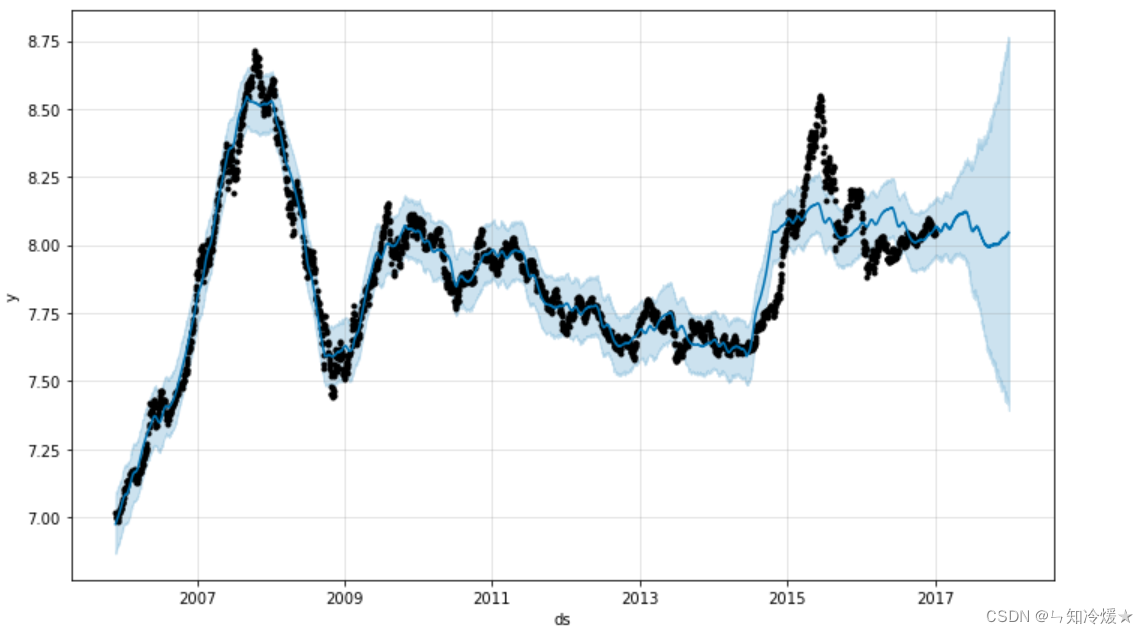
7-1-6、 Compare the predicted value with the real value
#  test , hold ds Column , namely data_series Column set as index column
df_test = df_test.set_index('ds')
#  Take out the predicted data ds Column , Predicted value column yhat, The same ds Column set as index column .
forecast = forecast[['ds','yhat']].set_index('ds')
#  Convert the data back , Because I passed before log function
df_test['y'] = np.exp(df_test['y'])
forecast['yhat'] = np.exp(forecast['yhat'])

# join: Join by index ,
# dropna: Be able to find DataFrame Null value of type data ( Missing value ), The line where the null value is located / After column deletion , New DataFrame Return as return value .
df_all = forecast.join(df_test).dropna()
df_all.plot()
#  Set the small mark in the upper left corner
plt.legend(['true', 'yhat'])
plt.show()
Contrast figure :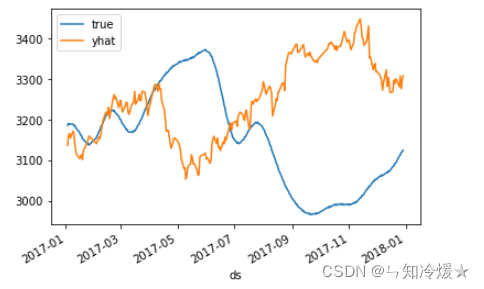
summary : Without adding any trick The long-term prediction effect of is very poor , But it can be seen that the accuracy of short-term prediction is still good .
7-2、 Battery Diviner
7-2-1、 Import related libraries
import pandas as pd
from prophet import Prophet
import numpy as np
import math
import matplotlib.pyplot as plt
7-2-2、 Reading data
#  Reading data
df = pd.read_csv('./energy.csv')
#  Change column name , Change to Prophet Specified column name ds and y
dd = df.rename(columns={
    'Datetime':'ds','AEP_MW':'y'})
#  Be careful :Prophet The model has requirements for data format , The date field must be datetime Format , Through here pd.to_datetime To switch .
dd['ds'] = pd.to_datetime(dd['ds'])
#  The data is read as hourly data , We need to aggregate it into days of data
dd = dd.set_index('ds').resample('D').sum().reset_index()
dd
data : On the left is the date , On the right is the corresponding electricity consumption of the day .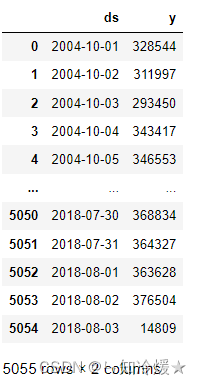
7-2-3、 Data preprocessing and the division of training set and test set .
#  Divide the data , It is divided into training set and verification set , The forecast data is set for the next month
df_train = dd[:5025]
df_test = dd[5025:]
df_train.plot('ds', ['y'])
current df_train As shown in the figure :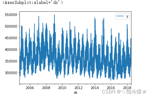
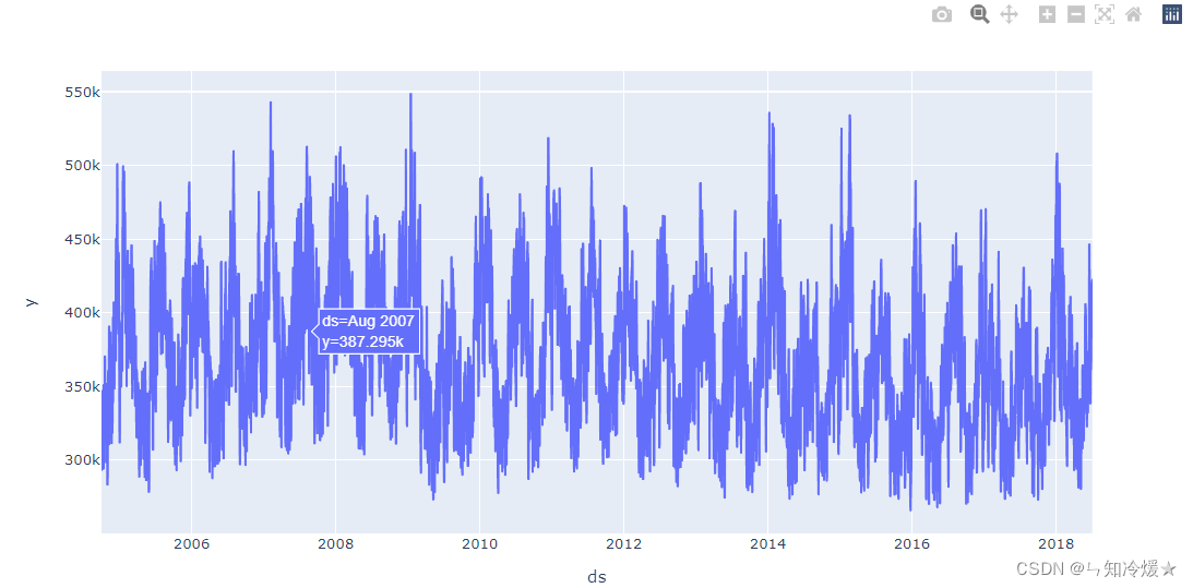
Observation data : Import a nice package , The painting is more beautiful
import plotly.express as px

fig = px.line(df_train, x="ds", y="y")
fig.show()
7-2-4、 Instantiation Prophet object , And through fit To train the model
#  Changes in data will be affected by seasons 、 Zhou 、 The influence of heaven , There is a certain regularity , So we set these three parameters to True
m = Prophet(yearly_seasonality=True, weekly_seasonality=True, daily_seasonality=True)
#  Adopt the Chinese holiday mode , Other parameters remain the default
m.add_country_holidays(country_name="CN")
m.fit(df_train)
# make_future_dataframe:  The function is to tell the model how long we want to predict , And what is the period of time . I'm going to set it to 30, That is, the data that predicts a month .
future = m.make_future_dataframe(periods=30, freq='D')
#  To make predictions , Return the predicted result forecast
forecast = model.predict(future)
# forecast['additive_terms'] = forecast['weekly'] + forecast['yearly'];
#  Yes :forecast['yhat']  = forecast['trend'] +  forecast['additive_terms'] .
#  therefore :forecast['yhat']  = forecast['trend'] +forecast['weekly'] + forecast['yearly'].
#  If there are holidays , Then there will be forecast['yhat']  = forecast['trend'] +forecast['weekly'] + forecast['yearly'] + forecast['holidays'].
forecast
forecast Express :Dataframe It contains a lot of information about the predicted results , among yhat Indicates the predicted result .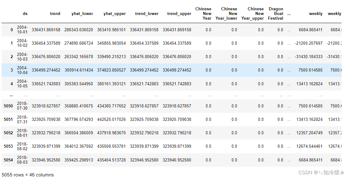
7-2-5、 Data visualization
# Visual operation of data models , Black dots represent real data , The blue line indicates the prediction result . The blue area indicates the upper and lower prediction limits under a certain degree of confidence .
m.plot(forecast)
plt.show()
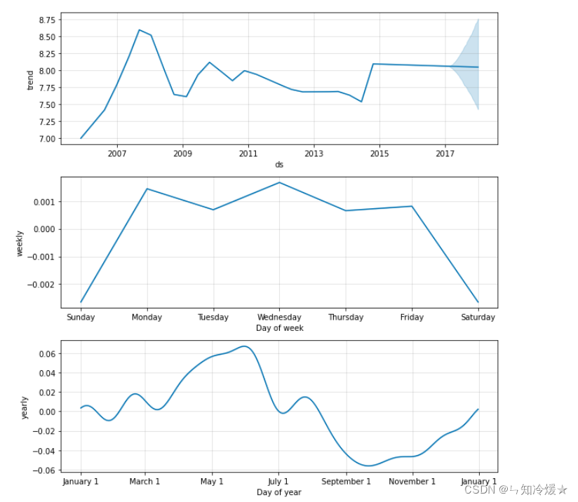
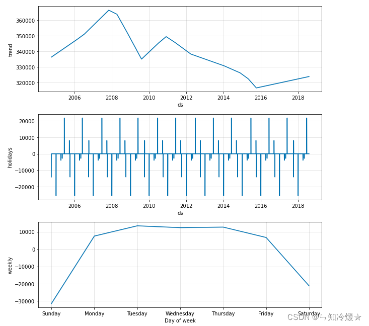
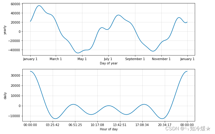
# adopt plot_componets() It can realize the year of data 、 month 、 Visualization of trends in different time periods of the week .
m.plot_components(forecast);
Data visualization :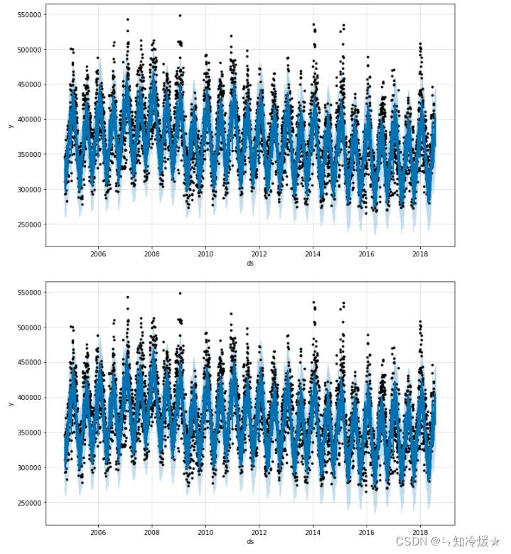
7-2-6、 Compare the predicted value with the real value
#  test
#  test , hold ds Column , namely data_series Column set as index column
df_test = df_test.set_index('ds')

#  Take out the predicted data ds Column , Predicted value column yhat, The same ds Column set as index column .
forecast = forecast[['ds','yhat']].set_index('ds')

# df_test['y'] = np.exp(df_test['y'])
# forecast['yhat'] = np.exp(forecast['yhat'])

# join: Join by index ,
# dropna: Be able to find DataFrame Null value of type data ( Missing value ), The line where the null value is located / After column deletion , New DataFrame Return as return value .
df_all = forecast.join(df_test).dropna()
df_all.plot()
#  Set the small mark in the upper left corner
plt.legend(['true', 'yhat'])
plt.show()
Contrast figure :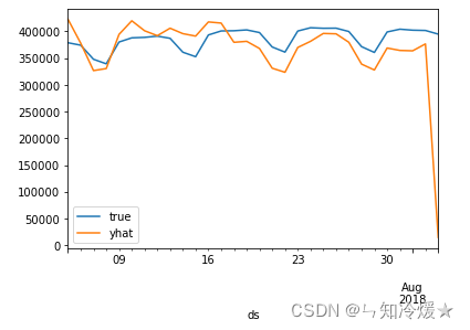
summary : Compared to stock forecasts , Only predict the power consumption in the next month , It can be said that it is very accurate , The basic trends are fitted .
7-2-7、 Model to evaluate
Model to evaluate : Evaluate the accuracy of the model , adopt RMSE( Mean square error ) To measure y And pre The degree of difference between , The smaller the value. , It indicates that the better the fitting degree is
train_len = len(df_train["y"])
rmse = np.sqrt(sum((df_train["y"] - forecast["yhat"].head(train_len)) ** 2) / train_len)
print('RMSE Error in forecasts = {}'.format(round(rmse, 2)))
7-2-7、 Model storage
Model storage : The above process realizes Prophet Model structures, , But considering the future, we will reuse the model trained by this historical data , So we need to store the model locally , And import it when necessary , Use pickle To save the model
import pickle

#  Model preservation
with open('../models_pickle/automl.pkl', 'wb') as f:
    pickle.dump(model, f, pickle.HIGHEST_PROTOCOL)

#  Model reading
# with open('prophet_model.json', 'r') as md:
# model = model_from_json(json.load(md))
8、 ... and 、 Other matters needing attention
8-1、 Holiday settings .
#  sometimes , Because of the double 11 or some special holidays , We can set some days as holidays , And set its front and back influence range , That is to say  lower_window  and  upper_window.
playoffs = pd.DataFrame({

  'holiday': 'playoff',
  'ds': pd.to_datetime(['2008-01-13', '2009-01-03', '2010-01-16',
                        '2010-01-24', '2010-02-07', '2011-01-08',
                        '2013-01-12', '2014-01-12', '2014-01-19',
                        '2014-02-02', '2015-01-11', '2016-01-17',
                        '2016-01-24', '2016-02-07']),
  'lower_window': 0,
  'upper_window': 1,
})
superbowls = pd.DataFrame({

  'holiday': 'superbowl',
  'ds': pd.to_datetime(['2010-02-07', '2014-02-02', '2016-02-07']),
  'lower_window': 0,
  'upper_window': 1,
})
holidays = pd.concat((playoffs, superbowls))

m = Prophet(holidays=holidays, holidays_prior_scale=10.0)
Reference article :
First time to know Prophet Model ( One )-- Theory Chapter .
Reading : One comes from Facebook Team's large-scale time series prediction algorithm ( attach github link ).
【python quantitative 】 take Facebook Of Prophet Algorithm for stock price prediction .
exclusive | I'll teach you how to use Python Of Prophet Library for time series prediction .
Facebook Time series prediction algorithm Prophet The study of .
Official website .
The paper .
Time series model Prophet Use to explain in detail .
Data anomaly detection :
「 Experience 」 how 30min Internal row finds out the reason for the indicator change .
「 Experience 」 Index change troubleshooting ,3 A method to quickly locate the abnormal dimension .
「 Experience 」 Index change troubleshooting , How to quantify the contribution to the market .
summary
边栏推荐
- Wchars, coding, standards and portability - wchars, encodings, standards and portability
- 队列的实现
- C language college laboratory reservation registration system
- Redis的五种数据结构
- Jerry's watch reading setting status [chapter]
- [swoole series 2.1] run the swoole first
- 华为0基金会——图片整理
- SQL优化问题的简述
- 关于这次通信故障,我想多说几句…
- F200 - UAV equipped with domestic open source flight control system based on Model Design
猜你喜欢
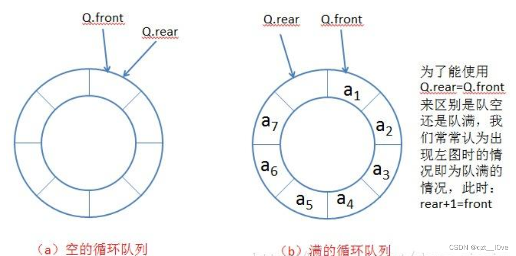
队列的实现
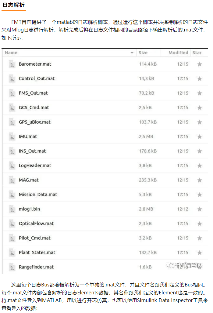
FMT open source self driving instrument | FMT middleware: a high real-time distributed log module Mlog
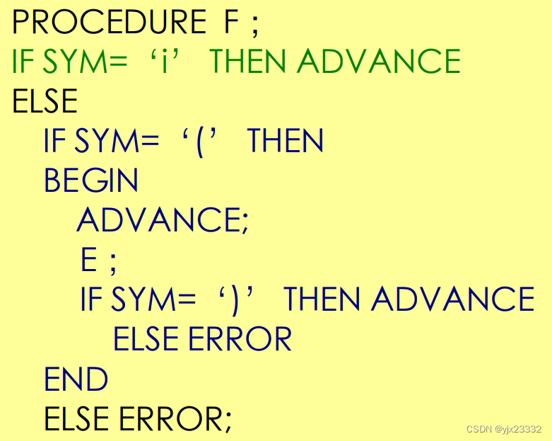
Compilation principle - top-down analysis and recursive descent analysis construction (notes)
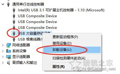
win10系统下插入U盘有声音提示却不显示盘符
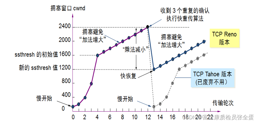
Transport layer congestion control - slow start and congestion avoidance, fast retransmission, fast recovery
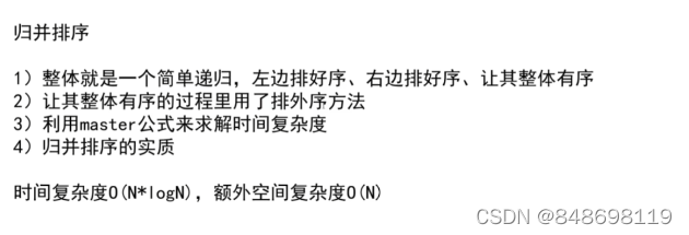
Recursive way
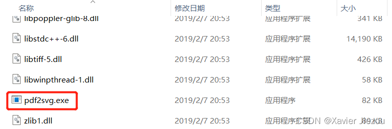
简单易用的PDF转SVG程序
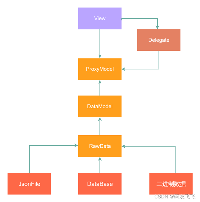
QT中Model-View-Delegate委托代理机制用法介绍
![Jerry's updated equipment resource document [chapter]](/img/6c/17bd69b34c7b1bae32604977f6bc48.jpg)
Jerry's updated equipment resource document [chapter]
模板于泛型编程之declval
随机推荐
Kill -9 system call used by PID to kill process
首先看K一个难看的数字
【剑指 Offer】 60. n个骰子的点数
F200 - UAV equipped with domestic open source flight control system based on Model Design
HMS core machine learning service creates a new "sound" state of simultaneous interpreting translation, and AI makes international exchanges smoother
Maixll dock camera usage
Jerry's updated equipment resource document [chapter]
Cocos2d Lua 越来越小样本 内存游戏
高精度运算
Redis的五种数据结构
Distiller les connaissances du modèle interactif! L'Université de technologie de Chine & meituan propose Virt, qui a à la fois l'efficacité du modèle à deux tours et la performance du modèle interacti
Nodejs developer roadmap 2022 zero foundation Learning Guide
Jerry's watch deletes the existing dial file [chapter]
Rb157-asemi rectifier bridge RB157
std::true_type和std::false_type
Reprint: defect detection technology of industrial components based on deep learning
UDP协议:因性善而简单,难免碰到“城会玩”
Jielizhi obtains the customized background information corresponding to the specified dial [chapter]
重磅硬核 | 一文聊透对象在 JVM 中的内存布局,以及内存对齐和压缩指针的原理及应用
2022暑期项目实训(三)