Realizing deep learning framework from zero -- Introduction to neural network

introduction

In line with “ Everything I can't create , I can't understand ” Thought , This series The article will be based on pure Python as well as NumPy Create your own deep learning framework from zero , The framework is similar PyTorch It can realize automatic derivation .

Deep understanding and deep learning , The experience of creating from scratch is very important , From an understandable point of view , Try not to use an external complete framework , Implement the model we want . This series The purpose of this article is through such a process , Let us grasp the underlying realization of deep learning , Instead of just being a switchman .
This series is first official account of WeChat public. ：JavaNLP

In our last article, we learned about the concept of neuron , In this article, let's learn about neural networks (Neural Network) Basic knowledge of .

Exclusive or questions

Let's first look at the famous XOR problem , This problem has led to the decade low point of neural network research .

The following pictures in this article are from nlp3

Exclusive or questions (XOR problem)： Enter two Boolean values (0 or 1), When the two values are different, the output is 1, Otherwise, the output is 0.

Pictured above , Suppose the input is x1、x2, The output is y.

Before introducing Neural Networks , Let's first look at the perceptron (perceptron), The perceptron can be likened to a neuron , But it doesn't have a nonlinear activation function .

Perceptron is a binary classifier ( With weight $w$ And offset $b$), Put the input $x$( Real valued vector ) Map to binary output . The output can be recorded as 0 or 1, Or rather, -1 and +1. The calculation method of the perceptron is as follows ：
$$y=\{\begin{array}{ll}0,& \text{if w⋅x+b≤0 }\\ 1,& \text{if w⋅x+b>0 }\end{array}\text{\hspace{1em}(1)}$$
We can easily build a system that can calculate and calculate (AND) And or operation (OR) Our perceptron ：

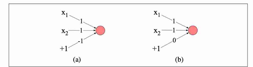
The figure above shows the implementation and (a) And or (b) The perceptron of computation . The inputs are $x_1,x_2$​. The value on the line above represents the weight or offset .

such as (a) by $x_1+x_2-1$, Input is $1,1$ when , The result is $1>0$, So the output $y=1$.

Addition and operation (AND) and Or operations (OR), XOR operation is also important .

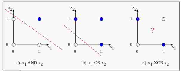
But we can't realize XOR operation through a perceptron . Because the perceptron is a linear classifier , For 2D input $x_1$ and $x_2$, Perceptron equation $w_1{x}_1+w_2{x}_2+b=0$ It's an equation of a straight line , This line serves as the decision boundary in two-dimensional space , One side represents output $0$, The output of the other side is $1$.

The following figure shows the possible logic inputs （00、01、10 and 11）, And by AND and OR A line drawn by a set of possible parameters of the classifier . But we can't draw a line that will XOR The true example of （01 and 10） And negative examples （00 and 11） Distinguish . We said XOR Not a linearly separable function .

Solution ： neural network

Although the XOR function cannot be represented by a single perceptron , But it can be represented by a hierarchical network based on perceptron units . Let's see how to use two layers ReLU Unit computation XOR problem .

There are three in the two-tier network ReLU unit , Namely $h_1,h_2$ and $y_1$. The number on the edge represents the weight of each unit $w$, Gray directed edges represent offsets .

Assume that the input $x=[0,0]$, We calculated

It's used here ReLU Activation function , therefore $h_2$ The output of is $0$, You can verify other inputs by yourself .

In this example, we fix the weight value , But in fact, the weight of neural network is automatically learned through back-propagation algorithm .

Now let me learn about the most common neural networks .

Feedforward neural networks

Feedforward neural networks ( Feedforward Neural Networks,FNN) It is a multi-layer network without circulation that spreads layer by layer . For historical reasons , Multilayer feedforward network , Also known as multilayer perceptron (multi-layer perceptron,MLP). But this is a technical misnomer , Because neurons in modern multi-layer networks are not perception machines ( The perceptron is purely linear , But neurons in modern networks have nonlinear activation functions ).

Simple ( Two layers of ) Feedforward networks have three types of nodes ： input unit 、 Hidden units and output units , As shown in the figure below .

Input layer $x$ It usually represents a vector composed of multiple scalars ; The core of neural network is hidden layer $h$, By hidden cells $h_i$ form , Each hidden unit is the neuron we learned earlier , The hidden layer calculates the weighted sum of its input and applies a nonlinear function . In the standard architecture , Each layer is fully connected ( Every neuron is connected to every input ).

Why is this a two-layer neural network , Because when we describe the number of layers , The input layer is usually ignored .

Note that each hidden cell has a weight parameter and an offset . We do this by putting each unit $i$ The weight vector and deviation of are combined into the weight matrix of the whole layer $W$ And the bias vector $B$ To represent the parameters of the entire hidden layer . Weight matrices $W$ Every element in $W_{ji}$ Says from the first $i$ Input units $x_i$ To the first $j$ Hidden units $h_j$ The weight of the connection .

Use a matrix $W$ The advantage of representing the weight of the entire layer is , Now through simple matrix operation , The hidden layer calculation of feedforward network can be completed very effectively . actually , There are only three steps to calculate ： Multiply the weight matrix by the input vector $x$, Add the offset vector $b$, Then apply the activation function $g$( such as Sigmoid、tanh or ReLU etc. ).

Hidden layer output , vector $h$, Therefore, it can be calculated as follows ( Let's suppose we use Sigmoid As an activation function )：
$$h=\sigma (Wx+b)\text{\hspace{1em}(2)}$$

Sometimes , We also use $\sigma$ It generally refers to any activation function , Not just Sigmoid.

$Wx+b$ The result is a vector , therefore $\sigma$ Apply to this vector .

Now let's introduce some commonly used marks , To better describe the following content .

In this case , We call the input layer the... Of the network $0$ layer (layer 0),$n_0$ Indicates the number of inputs in the input layer , therefore $x$ The dimension is $n_0$ Real vector of , Or formally $x\in {\mathbb{R}}^{n_0}$ The column vector $[n_0\times 1]$; We call the hidden layer $1$ layer (layer 1), The output layer is $2$ layer (layer 2); Dimensions of hidden layers ( The number of cells in the hidden layer ) yes $n_1$, therefore $h\in {\mathbb{R}}^{n_1}$, meanwhile $b\in {\mathbb{R}}^{n_1}$( Because each hidden cell has an offset ); Then the weight matrix $W$ The dimension of is $W\in {\mathbb{R}}^{n_1\times n_0}$( Combine the formula $(2)$).

So the formula $(2)$ An output in $h_j$, It can be expressed as $h_j=\sigma ({\sum }_{i=0}^{n_0}{W}_{ji}{x}_i+b_j)$.

Through the hidden layer , We set the dimension as $n_0$ The input vector of is expressed as dimension $n_1$ The hidden vector of , Then it is passed to the output layer to calculate the final output . The dimension of the output depends on the actual problem , For example, the regression problem is a real value ( Only one output ). But the common problem is classification . If it is a second category , Then the dimension of the output layer is $2$, Output unit ( Output node ) Only two. ; If it's multi classification , Then there are multiple output units .

Let's look at what happened in the output layer , The output layer also has a weight matrix ($U$),( There is no weight except for the input layer , This is one of the reasons why the input layer does not calculate the number of layers ), But some model output layers are not biased $b$ Of , So the weight matrix $U$ Directly with its input vector $h$ Multiply to get intermediate output $z$:
$$z=Uh\text{\hspace{1em}(3)}$$
The output layer has $n_2$ Output nodes , therefore $z\in {\mathbb{R}}^{n_2}$, Weight matrices $U\in {\mathbb{R}}^{n_2\times n_1}$, among $U_{ij}$ Is from the hidden layer $j$ Units to output layer $i$ Weight of units .

Be careful , there $z$ It's a real vector , Usually not the final output , For the classification model , We need to convert it into a probability distribution .

There is a very convenient function to normalize the vector of real numbers (normalizing) Is the probability distribution , The function is Softmax. Suppose the given dimension is $d$ Vector $z$,Softmax Defined as ：
$$\text{softmax}(z_i)=\frac{\exp (z_i)}{{\sum }_{j=1}^d\exp (z_j)}1\le i\le d\text{\hspace{1em}(4)}$$
That is, we can regard a neural network classifier with a hidden layer as building a vector $h$, It is a vector representation of the input , Then on the network $h$ Multiple logistic regression of running Standards . by comparison , Features in logistic regression are mainly designed manually through feature templates . So neural networks are like Softmax Logical regression , But the advantage is ：(a) There can be more layers , Because deep neural networks are like layer after layer of logistic regression classifiers ;(b) There are many optional activation functions in the middle tier (tanh,ReLU,sigmoid) Not just sigmoid（ Although we may use $\sigma$ To represent any activation function ）; Features are not formed through feature templates , The layer in front of the network forms its own feature representation .

We can get the two-layer feedforward network in this example , Also known as single hidden layer feedforward network , The final expression of ：
$$\begin{array}{rl}h& =\sigma (Wx+b)\\ z& =Uh\\ y& =\text{softmax}(z)\end{array}\text{\hspace{1em}(5)}$$
among $x\in {\mathbb{R}}^{n_0},h\in {\mathbb{R}}^{n_1},b\in {\mathbb{R}}^{n_1},W\in {\mathbb{R}}^{n_1\times n_0},U\in {\mathbb{R}}^{n_2\times n_1}$, Then output the vector $y\in {\mathbb{R}}^{n_2}$. We call this network a two-layer neural network . therefore , So to speak , Logistic regression is a layer of network . When resources can support , We can freely deepen the number of layers of the feedforward network , In this way, we can get the real deep neural network .

A more common notation indicates

Let's introduce some more common marks ,Andrew Ng This set of representation is also used . say concretely , Use the superscript in square brackets to indicate the number of layers , From the input layer 0 Start .

therefore ,$W^{[1]}$ Express ( first ) Weight matrix of hidden layer ,$b^{[1]}$ Express ( first ) The offset vector of the hidden layer ;$n_j$ Will denote the second $j$ Number of units in the layer ;$g(\cdot )$ To represent the activation function , The middle tier often uses ReLU or tanh Activation function , The output layer is often softmax;$a^{[i]}$ To represent the $i$ Layer output ,$z^{[i]}$ Express $W^{[i]}{a}^{[i-1]}+b^{[i]}$; The first 0 Layer is the input layer , So we will enter more generally $x$ be called $a^{[0]}$.

In this way, we rephrase the above single hidden layer feedforward network as ：
$$\begin{array}{rl}{z}^{[1]}& =W^{[1]}{a}^{[0]}+b^{[1]}\\ a^{[1]}& =g^{[1]}(z^{[1]})\\ z^{[2]}& =W^{[2]}{a}^{[1]}+b^{[2]}\\ a^{[2]}& =g^{[2]}(z^{[2]})\\ \hat{y}& =a^{[2]}\end{array}\text{\hspace{1em}(6)}$$

Replace the offset unit mark

In order to simplify the description of the network , We can omit the explicit description of bias $b$. So , We add a virtual node to each layer $a_0$, Its value will always be $1$. therefore , Input layer $0$ The layer will have virtual nodes $a_0^{[0]}=1$, layer $1$ Will have $a_0^{[1]}=1$, And so on . This virtual node still has an associated weight , This weight represents the deviation value $b$, For example, take the following equation ：
$$h=\sigma (Wx+b)$$
Replace with ：
$$h=\sigma (Wx)\text{\hspace{1em}(7)}$$
But now $x$ Vectors are not $n_0$ It's worth , Turned into $n_0+1$ It's worth , Include fixed values $x_0=1$, This becomes $x=x_0,\cdots ,x_{n_0}$. We can change the calculation $h_j$ The way , from ：
$$h_j=\sigma \left(\sum _{i=1}^{n_0}{W}_{ji}{x}_i+b_j\right)\text{\hspace{1em}(8)}$$
Turned into ：
$$h_j=\sigma \left(\sum _{i=0}^{n_0}{W}_{ji}{x}_i\right)\text{\hspace{1em}(9)}$$
Among them $W_{j0}$ To replace the $b_j$, We can also simplify the drawing ：

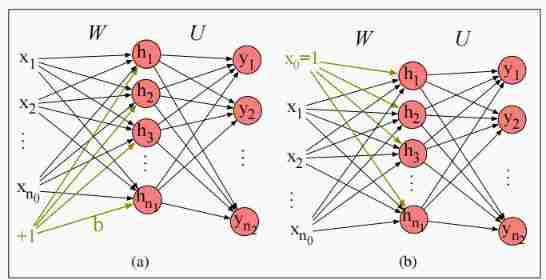
From the left of the above figure $(a)$ Simplified to the right $(b)$.

References

1. Speech and Language Processing