当前位置:网站首页>近段时间天气暴热,所以采集北上广深去年天气数据,制作可视化图看下
近段时间天气暴热,所以采集北上广深去年天气数据,制作可视化图看下
2022-07-02 03:35:00 【松鼠爱吃饼干】
前言
最近天气异常暴热,看到某些地方地表温度居然达到70°,这就离谱
所以就想采集一下天气的数据,做个可视化图,回忆一下去年的天气情况

开发环境
- python 3.8 运行代码
- pycharm 2021.2 辅助敲代码
- requests 第三方模块
天气数据采集
1. 发送请求
url = 'https://tianqi.2345.com/Pc/GetHistory?areaInfo%5BareaId%5D=54511&areaInfo%5BareaType%5D=2&date%5Byear%5D=2022&date%5Bmonth%5D=5'
response = requests.get(url)
print(response)
返回<Response [200]>: 请求成功

2. 获取数据
print(response.json())

3. 解析数据 天气信息提取出来
结构化数据解析:Python字典取值
非结构化数据解析:网页结构
json_data = response.json()
html_data = json_data['data']
select = parsel.Selector(html_data)
trs = select.css('table tr')
for tr in trs[1:]:
    # 网页结构
    # html网页 <td>asdfwaefaewfweafwaef</td> <a></a> <div></div>
    # ::text: 我需要这个 标签里面的文本内容
    td = tr.css('td::text').getall()
    print(td)
4. 保存数据
with open('天气数据.csv', encoding='utf-8', mode='a', newline='') as f:
    csv_writer = csv.writer(f)
    csv_writer.writerow(td)


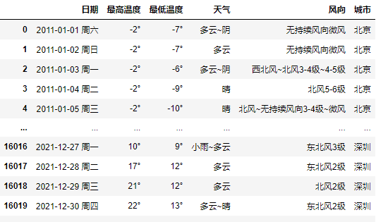
数据可视化效果
读取数据
data = pd.read_csv('天气数据.csv')
data
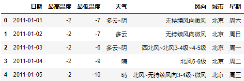
分割日期/星期
data[['日期','星期']] = data['日期'].str.split(' ',expand=True,n=1)
data

去除多余字符
data[['最高温度','最低温度']] = data[['最高温度','最低温度']].apply(lambda x: x.str.replace('°',''))
data.head()
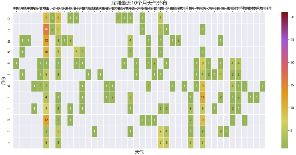
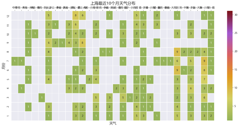
北上广深2021年10月份天气热力图分布
import matplotlib.pyplot as plt
import matplotlib.colors as mcolors
import seaborn as sns

#设置全局默认字体 为 雅黑
plt.rcParams['font.family'] = ['Microsoft YaHei']
# 设置全局轴标签字典大小
plt.rcParams["axes.labelsize"] = 14
# 设置背景
sns.set_style("darkgrid",{
    "font.family":['Microsoft YaHei', 'SimHei']})
# 设置画布长宽 和 dpi
plt.figure(figsize=(18,8),dpi=100)
# 自定义色卡
cmap = mcolors.LinearSegmentedColormap.from_list("n",['#95B359','#D3CF63','#E0991D','#D96161','#A257D0','#7B1216'])
# 绘制热力图

ax = sns.heatmap(data_pivot, cmap=cmap, vmax=30,
                 annot=True, # 热力图上显示数值
                 linewidths=0.5,
                )
# 将x轴刻度放在最上面
ax.xaxis.set_ticks_position('top')
plt.title('北京最近10个月天气分布',fontsize=16) #图片标题文本和字体大小
plt.show()


北京2021年每日最高最低温度变化
color0 = ['#FF76A2','#24ACE6']
color_js0 = """new echarts.graphic.LinearGradient(0, 1, 0, 0, [{offset: 0, color: '#FFC0CB'}, {offset: 1, color: '#ed1941'}], false)"""
color_js1 = """new echarts.graphic.LinearGradient(0, 1, 0, 0, [{offset: 0, color: '#FFFFFF'}, {offset: 1, color: '#009ad6'}], false)"""

tl = Timeline()
for i in range(0,len(data_bj)):
    coordy_high = list(data_bj['最高温度'])[i]
    coordx = list(data_bj['日期'])[i]
    coordy_low = list(data_bj['最低温度'])[i]
    x_max = list(data_bj['日期'])[i]+datetime.timedelta(days=10)
    y_max = int(max(list(data_bj['最高温度'])[0:i+1]))+3
    y_min = int(min(list(data_bj['最低温度'])[0:i+1]))-3
    title_date = list(data_bj['日期'])[i].strftime('%Y-%m-%d')
    c = (
        Line(
            init_opts=opts.InitOpts(
            theme='dark',
            #设置动画
            animation_opts=opts.AnimationOpts(animation_delay_update=800),#(animation_delay=1000, animation_easing="elasticOut"),
            #设置宽度、高度
            width='1500px',
            height='900px', )
        )
        .add_xaxis(list(data_bj['日期'])[0:i])
        .add_yaxis(
            series_name="",
            y_axis=list(data_bj['最高温度'])[0:i], is_smooth=True,is_symbol_show=False,
            linestyle_opts={

                   'normal': {

                       'width': 3,
                       'shadowColor': 'rgba(0, 0, 0, 0.5)',
                       'shadowBlur': 5,
                       'shadowOffsetY': 10,
                       'shadowOffsetX': 10,
                       'curve': 0.5,
                       'color': JsCode(color_js0)
                   }
               },
            itemstyle_opts={

            "normal": {

                "color": JsCode(
                    """new echarts.graphic.LinearGradient(0, 0, 0, 1, [{ offset: 0, color: '#ed1941' }, { offset: 1, color: '#009ad6' }], false)"""
                ),
                "barBorderRadius": [45, 45, 45, 45],
                "shadowColor": "rgb(0, 160, 221)",
            }
        },

        )
        .add_yaxis(
            series_name="",
            y_axis=list(data_bj['最低温度'])[0:i], is_smooth=True,is_symbol_show=False,
# linestyle_opts=opts.LineStyleOpts(color=color0[1],width=3),
            itemstyle_opts=opts.ItemStyleOpts(color=JsCode(color_js1)),
            linestyle_opts={

                   'normal': {

                       'width': 3,
                       'shadowColor': 'rgba(0, 0, 0, 0.5)',
                       'shadowBlur': 5,
                       'shadowOffsetY': 10,
                       'shadowOffsetX': 10,
                       'curve': 0.5,
                       'color': JsCode(color_js1)
                   }
               },
        )
        .set_global_opts(
            title_opts=opts.TitleOpts("北京2021年每日最高最低温度变化\n\n{}".format(title_date),pos_left=330,padding=[30,20]),
            xaxis_opts=opts.AxisOpts(type_="time",max_=x_max),#, interval=10,min_=i-5,split_number=20,axistick_opts=opts.AxisTickOpts(length=2500),axisline_opts=opts.AxisLineOpts(linestyle_opts=opts.LineStyleOpts(color="grey"))
            yaxis_opts=opts.AxisOpts(min_=y_min,max_=y_max),#坐标轴颜色,axisline_opts=opts.AxisLineOpts(linestyle_opts=opts.LineStyleOpts(color="grey"))
        )
    )
    tl.add(c, "{}".format(list(data_bj['日期'])[i]))
    tl.add_schema(
        axis_type='time',
        play_interval=100,  # 表示播放的速度
        pos_bottom="-29px",
        is_loop_play=False, # 是否循环播放
        width="780px",
        pos_left='30px',
        is_auto_play=True,  # 是否自动播放。
        is_timeline_show=False)
tl.render_notebook()

北上广深10月份每日最高气温变化
# 背景色
background_color_js = (
    "new echarts.graphic.LinearGradient(0, 0, 0, 1, "
    "[{offset: 0, color: '#c86589'}, {offset: 1, color: '#06a7ff'}], false)"
)

# 线条样式
linestyle_dic = {
     'normal': {

                    'width': 4,
                    'shadowColor': '#696969',
                    'shadowBlur': 10,
                    'shadowOffsetY': 10,
                    'shadowOffsetX': 10,
                    }
                }

timeline = Timeline(init_opts=opts.InitOpts(bg_color=JsCode(background_color_js),
                                            width='980px',height='600px'))


bj, gz, sh, sz= [], [], [], []
all_max = []
x_data = data_10[data_10['城市'] == '北京']['日'].tolist()
for d_time in range(len(x_data)):
    bj.append(data_10[(data_10['日'] == x_data[d_time]) & (data_10['城市']=='北京')]["最高温度"].values.tolist()[0])
    gz.append(data_10[(data_10['日'] == x_data[d_time]) & (data_10['城市']=='广州')]["最高温度"].values.tolist()[0])
    sh.append(data_10[(data_10['日'] == x_data[d_time]) & (data_10['城市']=='上海')]["最高温度"].values.tolist()[0])
    sz.append(data_10[(data_10['日'] == x_data[d_time]) & (data_10['城市']=='深圳')]["最高温度"].values.tolist()[0])

    line = (
        Line(init_opts=opts.InitOpts(bg_color=JsCode(background_color_js),
                                     width='980px',height='600px'))
        .add_xaxis(
            x_data,
                  )

        .add_yaxis(
            '北京',
            bj,
            symbol_size=5,
            is_smooth=True,
            is_hover_animation=True,
            label_opts=opts.LabelOpts(is_show=False),
        )

        .add_yaxis(
            '广州',
            gz,
            symbol_size=5,
            is_smooth=True,
            is_hover_animation=True,
            label_opts=opts.LabelOpts(is_show=False),
        )

        .add_yaxis(
            '上海',
            sh,
            symbol_size=5,
            is_smooth=True,
            is_hover_animation=True,
            label_opts=opts.LabelOpts(is_show=False),

        )

        .add_yaxis(
            '深圳',
            sz,
            symbol_size=5,
            is_smooth=True,
            is_hover_animation=True,
            label_opts=opts.LabelOpts(is_show=False),

        )

        .set_series_opts(linestyle_opts=linestyle_dic)
        .set_global_opts(
            title_opts=opts.TitleOpts(
                title='北上广深10月份最高气温变化趋势',
                pos_left='center',
                pos_top='2%',
                title_textstyle_opts=opts.TextStyleOpts(color='#DC143C', font_size=20)),

            tooltip_opts=opts.TooltipOpts(
                trigger="axis",
                axis_pointer_type="cross",
                background_color="rgba(245, 245, 245, 0.8)",
                border_width=1,
                border_color="#ccc",
                textstyle_opts=opts.TextStyleOpts(color="#000"),
        ),
            xaxis_opts=opts.AxisOpts(
# axislabel_opts=opts.LabelOpts(font_size=14, color='red'),
# axisline_opts=opts.AxisLineOpts(is_show=True,
# linestyle_opts=opts.LineStyleOpts(width=2, color='#DB7093'))
                is_show = False
            ),


            yaxis_opts=opts.AxisOpts(
                name='最高气温',
                is_scale=True,
# min_= int(min([gz[d_time],sh[d_time],sz[d_time],bj[d_time]])) - 10,
                max_= int(max([gz[d_time],sh[d_time],sz[d_time],bj[d_time]])) + 10,
                name_textstyle_opts=opts.TextStyleOpts(font_size=16,font_weight='bold',color='#5470c6'),
                axislabel_opts=opts.LabelOpts(font_size=13,color='#5470c6'),
                splitline_opts=opts.SplitLineOpts(is_show=True,
                                                  linestyle_opts=opts.LineStyleOpts(type_='dashed')),
                axisline_opts=opts.AxisLineOpts(is_show=True,
                                        linestyle_opts=opts.LineStyleOpts(width=2, color='#5470c6'))
            ),
            legend_opts=opts.LegendOpts(is_show=True, pos_right='1%', pos_top='2%',
                                        legend_icon='roundRect',orient = 'vertical'),
        ))

    timeline.add(line, '{}'.format(x_data[d_time]))

timeline.add_schema(
    play_interval=1000,          # 轮播速度
    is_timeline_show=True,      # 是否显示 timeline 组件
    is_auto_play=True,          # 是否自动播放
    pos_left="0",
    pos_right="0"
)
timeline.render_notebook()

边栏推荐
- In depth analysis of C language - variable error prone knowledge points # dry goods inventory #
- 初出茅庐市值1亿美金的监控产品Sentry体验与架构
- Oracle common SQL
- The page in H5 shows hidden execution events
- What do you know about stock selling skills and principles
- Generate random numbers that obey normal distribution
- PY3 link MySQL
- Detailed explanation of ThreadLocal
- UI (New ui:: MainWindow) troubleshooting
- Aaaaaaaaaaaa
猜你喜欢

Named block Verilog
Exchange rate query interface

MSI announced that its motherboard products will cancel all paper accessories
Detailed explanation of ThreadLocal

Halcon image rectification
![[untitled] basic operation of raspberry pie (2)](/img/b4/cac22c1691181c1b09fe9d98963dbf.jpg)
[untitled] basic operation of raspberry pie (2)

This article describes the step-by-step process of starting the NFT platform project
Knowing things by learning | self supervised learning helps improve the effect of content risk control

Discrimination between sap Hana, s/4hana and SAP BTP

Verilog state machine
随机推荐
高性能 低功耗Cortex-A53核心板 | i.MX8M Mini
[untitled] basic operation of raspberry pie (2)
JS generate random numbers
h5中的页面显示隐藏执行事件
蓝桥杯单片机第四届省赛
NLog使用
Uniapp uses canvas to generate posters and save them locally
Learn PWN from CTF wiki - ret2shellcode
终日乾乾,夕惕若厉
MySQL index, transaction and storage engine
[mv-3d] - multi view 3D target detection network
Verilog reg register, vector, integer, real, time register
How to establish its own NFT market platform in 2022
In wechat applet, the externally introduced JS is used in xwml for judgment and calculation
/silicosis/geo/GSE184854_scRNA-seq_mouse_lung_ccr2/GSE184854_RAW/GSM5598265_matrix_inflection_demult
Apple added the first iPad with lightning interface to the list of retro products
VS2010 plug-in nuget
Verilog parallel block implementation
Account management of MySQL
FFMpeg AVFrame 的概念.