当前位置:网站首页>Numpy quick start (V) -- Linear Algebra
Numpy quick start (V) -- Linear Algebra
2022-07-03 10:41:00 【serity】
Catalog
- This article is about NumPy The last in the quick start series .
- The matrix mentioned in this article refers to
np.arrayobject , Instead ofnp.matrixobject , The latter is no longer recommended . - NumPy in , The modules related to linear algebra are
np.linalg(linear algebra), We usually abbreviate it asLA, namely
from numpy import linalg as LA
One 、@ operator
Numpy in ,@ The operator can be used to calculate the product of two matrices :
A = np.array([[1, 2], [3, 4]])
B = np.array([[5, 6], [7, 8]])
print(A @ B)
# [[19 22]
# [43 50]]
np.matmul It can also be used to calculate the product of two matrices , But it is more recommended here @.
Two 、 Vector product and matrix product
| function | effect |
|---|---|
| np.inner(a, b) | a and b It's all One dimensional array ( vector ); Calculate the of two vectors Inner product |
| np.outer(a, b) | Calculate the of two vectors Exoproduct |
| np.kron(a, b) | Calculate the Kronecker's product |
| LA.matrix_power(A, n) | A A A yes Matrix ; Calculation A n A^n An |
2.1 np.inner()
set up a a a and b b b Are the two ( Column ) vector , be np.inner(a, b) amount to a T b a^{\mathrm T}b aTb.
a = np.array([1, 2, 3])
b = np.array([3, 2, 1])
print(np.inner(a, b))
# 10
2.2 np.outer()
set up a a a and b b b Are the two ( Column ) vector , be np.outer(a, b) amount to a b T ab^{\mathrm T} abT.
a = np.array([1, 2, 3])
b = np.array([3, 2, 1])
print(np.outer(a, b))
# [[3 2 1]
# [6 4 2]
# [9 6 3]]
2.3 np.kron()
For the definition of Kronecker product, please refer to Wikipedia. Kronecker product.
In most cases, we calculate the Kronecker product of two matrices , set up A A A and B B B It's two matrices , be np.kron(a, b) amount to A ⊗ B A\otimes B A⊗B.
A = np.array([[1, 2], [3, 4]])
B = np.array([[0, 5], [6, 7]])
print(np.kron(A, B))
# [[ 0 5 0 10]
# [ 6 7 12 14]
# [ 0 15 0 20]
# [18 21 24 28]]
2.4 LA.matrix_power()
We use nilpotent matrix to observe the effect :
A = np.eye(4, k=1)
print(A)
# [[0. 1. 0. 0.]
# [0. 0. 1. 0.]
# [0. 0. 0. 1.]
# [0. 0. 0. 0.]]
print(LA.matrix_power(A, 2))
# [[0. 0. 1. 0.]
# [0. 0. 0. 1.]
# [0. 0. 0. 0.]
# [0. 0. 0. 0.]]
print(LA.matrix_power(A, 3))
# [[0. 0. 0. 1.]
# [0. 0. 0. 0.]
# [0. 0. 0. 0.]
# [0. 0. 0. 0.]]
print(LA.matrix_power(A, 4))
# [[0. 0. 0. 0.]
# [0. 0. 0. 0.]
# [0. 0. 0. 0.]
# [0. 0. 0. 0.]]
3、 ... and 、 determinant 、 Rank 、 trace 、 norm
| function | effect |
|---|---|
| LA.det(A) | Calculation of matrix A The determinant of |
| LA.matrix_rank(A) | Calculation of matrix A The rank of |
| np.trace(A) | Calculation of matrix A The trace of |
| LA.norm(a, ord=None) | ord Control norm ; Calculate the norm of a vector or matrix |
3.1 LA.det()
A = np.array([[1, 2], [3, 4]])
print(LA.det(A))
# -2.0000000000000004
3.2 LA.matrix_rank()
A = np.array([[1, 2], [3, 4]])
B = np.array([[1, 1], [1, 1]])
C = np.array([[0, 0], [0, 0]])
print(LA.matrix_rank(A))
print(LA.matrix_rank(B))
print(LA.matrix_rank(C))
# 2
# 1
# 0
3.3 np.trace()
A = np.identity(4)
print(np.trace(A))
# 4.0
3.4 LA.norm()
Before further explanation of usage , Let's first review the common norms of matrices and vectors :
| Matrix norm | expression |
|---|---|
| Frobenius norm | ∥ A ∥ F = ( ∑ i , j ∣ a i j ∣ 2 ) 1 / 2 \displaystyle\Vert A\Vert_F=\Big(\sum_{i,j}\mid \!a_{ij} \!\mid^2\Big)^{1/2} ∥A∥F=(i,j∑∣aij∣2)1/2 |
| 1 1 1 - norm | ∥ A ∥ 1 = max j ∑ i ∣ a i j ∣ \displaystyle \Vert A\Vert_1=\max_{j} \sum_i \mid \!a_{ij}\!\mid ∥A∥1=jmaxi∑∣aij∣ |
| 2 2 2 - norm | ∥ A ∥ 2 = λ m a x ( A H A ) \displaystyle \Vert A\Vert_2=\sqrt{\lambda_{max}(A^H A)} ∥A∥2=λmax(AHA) |
| ∞ \infty ∞ - norm | ∥ A ∥ ∞ = max i ∑ j ∣ a i j ∣ \displaystyle \Vert A\Vert_{\infty}=\max_{i} \sum_j\mid \!a_{ij}\!\mid ∥A∥∞=imaxj∑∣aij∣ |
| Kernel norm | ∥ A ∥ ∗ = t r ( A H A ) \displaystyle \Vert A\Vert_{*}=\mathrm{tr}(\sqrt{A^H A}) ∥A∥∗=tr(AHA) |
| Vector norm | expression |
|---|---|
| p p p norm ( 1 ≤ p < + ∞ 1\leq p<+\infty 1≤p<+∞) | ∥ x ∥ p = ( ∑ i ∣ x i ∣ p ) 1 / p \displaystyle\Vert \boldsymbol x\Vert_p=\Big(\sum_i\mid\!x_i\!\mid^p\Big)^{1/p} ∥x∥p=(i∑∣xi∣p)1/p |
| ∞ \infty ∞ - norm | ∥ x ∥ ∞ = max i ∣ x i ∣ \displaystyle\Vert \boldsymbol x\Vert_{\infty}=\max_i \mid\!x_i\!\mid ∥x∥∞=imax∣xi∣ |
Let's take a look at ord The common value of :
| ord | Matrix norm | Vector norm |
|---|---|---|
| None | Frobenius norm | 2 2 2 - norm |
| ‘nuc’ | Kernel norm | —— |
| inf | max(sum(abs(a), axis=1)) | max(abs(a)) |
| 1 | max(sum(abs(a), axis=0)) | sum(abs(a)) |
| 2 | 2 2 2 - norm | sum(abs(a) ∗ ∗ \ast\ast ∗∗ 2) ∗ ∗ \ast\ast ∗∗ (1./2) |
Specific code examples will not be given , Readers can practice by themselves if necessary .
Four 、 Eigenvalues and eigenvectors
| function | effect |
|---|---|
| LA.eig(A) | Computational matrix A Of The eigenvalue and Eigenvector |
| LA.eigh(A) | Calculation of matrix A Eigenvalues and eigenvectors (A yes Real symmetry Matrix or Hermite matrix ) |
| LA.eigvals(A) | Computational matrix A Of The eigenvalue |
| LA.eigvalsh(A) | Computational matrix A Of The eigenvalue (A yes Real symmetry Matrix or Hermite matrix ) |
4.1 LA.eig()
Let's first review the relevant definitions .
Only real number fields are considered here . set up A A A yes n n n Square matrix , If there is a constant λ \lambda λ And nonzero vectors x x x bring
A x = λ x Ax=\lambda x Ax=λx
said λ \lambda λ yes A A A Of The eigenvalue , x x x yes A A A Belong to characteristic value λ \lambda λ Of Eigenvector .
Do not consider repeated situations , A A A There must be n n n Eigenvalues , Write it down as λ 1 , ⋯ , λ n \lambda_1,\cdots,\lambda_n λ1,⋯,λn, The corresponding eigenvector is recorded as p 1 , ⋯ , p n \boldsymbol{p}_1, \cdots,\boldsymbol{p}_n p1,⋯,pn.
Make λ = [ λ 1 , ⋯ , λ n ] \boldsymbol{\lambda}=[\lambda_1,\cdots,\lambda_n] λ=[λ1,⋯,λn], P = [ p 1 , ⋯ , p n ] \boldsymbol{P}=[\boldsymbol{p}_1, \cdots,\boldsymbol{p}_n] P=[p1,⋯,pn], You know λ \boldsymbol{\lambda} λ It's a one-dimensional array , P \boldsymbol{P} P Is a two-dimensional array . Yes A A A Use LA.eig(A) Will return a Tuples ( λ , P ) (\boldsymbol{\lambda}, \boldsymbol{P}) (λ,P), We usually use two parameters w, v Receive :
A = np.diag((3, 2, 1))
w, v = LA.eig(A)
print(w)
# [3. 2. 1.]
print(v)
# [[1. 0. 0.]
# [0. 1. 0.]
# [0. 0. 1.]]
Combined with the above definition , We can see :
v[:, i]yes A A A Belong to characteristic valuew[i]Eigenvector of .
Let's take another example
A = np.array([
    [1, -1, 3],
    [0, 1, 2],
    [0, 0, 2]
])
w, v = LA.eig(A)
print(w)
# [1. 1. 2.]
print(v)
# [[1.00000000e+00 1.00000000e+00 4.08248290e-01]
# [0.00000000e+00 2.22044605e-16 8.16496581e-01]
# [0.00000000e+00 0.00000000e+00 4.08248290e-01]]
It is not difficult to see from the results that ∥ p i ∥ = 1 \Vert \boldsymbol{p}_i\Vert=1 ∥pi∥=1, That is, each eigenvector after return v[:, i] All are Standardization the . Besides , It can also be seen from the first example , Our eigenvalue list w It is not arranged from small to large .
4.2 LA.eigh()
The list of characteristic values returned by this function
wyes From small to large To arrange ( Real symmetry / The eigenvalue of Hermite matrix is always The set of real Numbers ).
For real symmetric matrix and Hermite matrix , Of course, we can also use LA.eig Calculate , But there is no doubt that LA.eigh It's better , Because it uses real symmetry / The properties of Hermite matrix thus Speed up the calculation .
Specific code examples will not be given , Readers can practice by themselves if necessary .
4.3 LA.eigvals()
This function only returns the list of characteristic values
w, Andwnot always It is arranged from small to large .
A = np.diag((3, 2, 1))
print(LA.eigvals(A))
# [3. 2. 1.]
4.4 LA.eigvalsh()
The list of characteristic values returned by this function
wyes From small to large To arrange .
Specific code examples will not be given , Readers can practice by themselves if necessary .
边栏推荐
- Simple real-time gesture recognition based on OpenCV (including code)
- Ut2014 supplementary learning notes
- An open source OA office automation system
- Leetcode刷题---278
- Leetcode刷题---832
- Leetcode刷题---283
- Ind kwf first week
- 熵值法求权重
- Inverse code of string (Jilin University postgraduate entrance examination question)
- Seata分布式事务失效,不生效(事务不回滚)的常见场景
猜你喜欢

Judging the connectivity of undirected graphs by the method of similar Union and set search
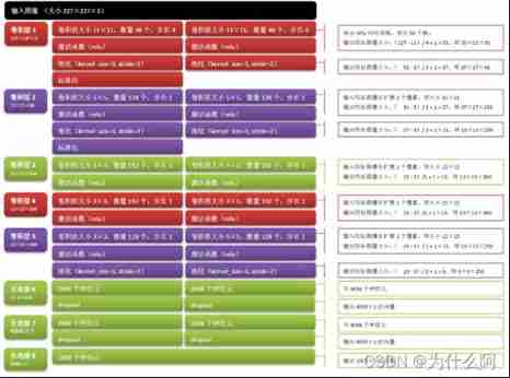
Handwritten digit recognition: CNN alexnet
![[untitled]](/img/41/adf5638e4a36417ce8dba3f2c4d9ed.jpg)
[untitled]

Jetson TX2 brush machine

GAOFAN Weibo app
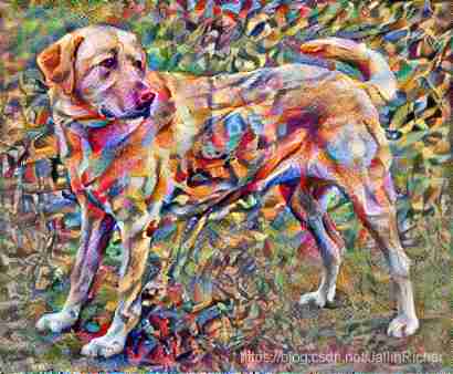
Tensorflow—Neural Style Transfer

MySQL reports an error "expression 1 of select list is not in group by claim and contains nonaggre" solution

Ind kwf first week
Ut2017 learning notes
Data classification: support vector machine
随机推荐
Install yolov3 (Anaconda)
[LZY learning notes -dive into deep learning] math preparation 2.5-2.7
深度学习入门之线性回归(PyTorch)
[LZY learning notes dive into deep learning] 3.1-3.3 principle and implementation of linear regression
Training effects of different data sets (yolov5)
OpenCV Error: Assertion failed (size.width>0 && size.height>0) in imshow
[untitled] numpy learning
Ut2012 learning notes
Leetcode skimming ---278
[combinatorial mathematics] pigeon's nest principle (simple form of pigeon's nest principle | simple form examples of pigeon's nest principle 1, 2, 3)
Leetcode skimming ---202
Ind FXL first week
Unity小组工程实践项目《最强外卖员》策划案&纠错文档
Tensorflow—Image segmentation
【SQL】一篇带你掌握SQL数据库的查询与修改相关操作
丢弃法Dropout(Pytorch)
A complete mall system
Adaptive Propagation Graph Convolutional Network
CSDN, I'm coming!
7、 Data definition language of MySQL (2)