当前位置:网站首页>Value Function Approximation
Value Function Approximation
2022-07-07 00:27:00 【Evergreen AAS】
Why do we need value function approximation ?
We mentioned various methods of calculating value functions before , For example, for MDP Known problems can be used Bellman The expectation equation obtains the value function ; about MDP The unknown , Can pass MC as well as TD Method to get the value function , Why do we need to approximate the value function again ?
In fact, so far , The value function calculation methods we introduced are obtained by looking up the table :
- Each state in the table s They all correspond to one V(s)
- Or every state - action
But for large MDP problem , The above methods will encounter bottlenecks :
- Too many MDP state 、 Actions need to be stored
- Calculating the value of each state alone is very time-consuming
Therefore, we need a method that can be applied to solve large MDP A general approach to the problem , This is the value function approximation method introduced in this paper . namely :
\hat{v}(s, \mathbf{w}) \approx v_{\pi}(s) \\ \text{or } \hat{q}(s, a, \mathbf{w}) \approx q_{\pi}(s, a)
So why can the value function approximation method solve large MDP problem ?
For large MDP The problem is , We can approximate that it is unrealistic that all its states and actions are sampled and calculated , So once we get the approximate value function , We can generalize those States and actions that have not appeared in historical experience or sampling (generalize).
There are many training methods for value function approximation , such as :
- Linear regression
- neural network
- Decision tree
- …
Besides , in the light of MDP Characteristics of the problem , The training function must be applicable to non static 、 Non independent identically distributed (non-i.i.d) The data of .
Incremental method
gradient descent
Approximation of the value function by random gradient descent
The objective function we optimize is to find a set of parameters w To minimize the least square error (MSE), namely :
J(\mathbf{w}) = E_{\pi}[(v_{\pi}(S) - \hat{v}(S, \mathbf{w}))^2]
Optimize by gradient descent method :
\begin{align} \Delta\mathbf{w} &=-\frac{1}{2}\alpha\triangledown_{\mathbf{w}}J(\mathbf{w})\\ &=\alpha E_{\pi}\Bigl[\Bigl(v_{\pi}(S) - \hat{v}(S, \mathbf{w})\Bigr)\triangledown_{\mathbf{w}}J(\mathbf{w})\Bigr] \end{align}
For random gradient descent (Stochastic Gradient Descent,SGD), The corresponding gradient :
\Delta\mathbf{w} = \alpha\underbrace{\Bigl(v_{\pi}(S) - \hat{v}(S, \mathbf{w})\Bigr)}_{\text{error}}\underbrace{\triangledown_{\mathbf{w}}\hat{v}(S, \mathbf{w})}_{\text{gradient}}
Value function approximation
The above formula requires a real strategic value function vπ(S)vπ(S) As the goal of learning (supervisor), But in RL There is no real strategic value function in , Only rewards. in application , We use it v~π~(S) Instead of target vπ(S):
- about MC,target by return G~t ~:
\Delta\mathbf{w}=\alpha\Bigl(G_t - \hat{v}(S_t, \mathbf{w})\Bigr)\triangledown_{\mathbf{w}}\hat{v}(S_t, \mathbf{w})
- about TD(0),target by TD target _{t+1}+\gamma\hat{v}(S_{t+1}, \mathbf{w}):
\Delta\mathbf{w}=\alpha\Bigl(R_{t+1} + \gamma\hat{v}(S_{t+1}, \mathbf{w})- \hat{v}(S_t, \mathbf{w})\Bigr)\triangledown_{\mathbf{w}}\hat{v}(S_t, \mathbf{w})
- about TD(λ),target by TD λ-return G_t^{\lambda}:
\Delta\mathbf{w}=\alpha\Bigl(G_t^{\lambda}- \hat{v}(S_t, \mathbf{w})\Bigr)\triangledown_{\mathbf{w}}\hat{v}(S_t, \mathbf{w})
After obtaining the approximation of the value function, you can control , The specific diagram is as follows :
The action value function is approximate
The action value function is approximate :
\hat{q}(S, A, \mathbf{w})\approx q_{\pi}(S, A)
Optimization objectives : To minimize the MSE
J(\mathbf{w}) = E_{\pi}[(q_{\pi}(S, A) - \hat{q}(S, A, \mathbf{w}))^2]
Use SGD Optimization :
\begin{align} \Delta\mathbf{w} &=-\frac{1}{2}\alpha\triangledown_{\mathbf{w}}J(\mathbf{w})\\ &=\alpha\Bigl(q_{\pi}(S, A)-\hat{q}_{\pi}(S, A, \mathbf{w})\Bigr) \triangledown_{\mathbf{w}}\hat{q}_{\pi}(S, A, \mathbf{w}) \end{align}
Batch method
Stochastic gradient descent SGD Simple , But the batch method can be based on agent Experience to better fit the value function .
Value function approximation
Optimization objectives : The problem solved by batch method is also \hat{v}(s, \mathbf{w})\approx v_{\pi}(s)
Experience set D It contains a series of pair:
D=\{<s_1, v_1^{\pi}>, <s_2, v_2^{\pi}>, ..., <s_T, v_T^{\pi}>\}
Fit according to the sum of minimized square errors \hat{v}(s, \mathbf{w}) and v~π~(s) , namely :
\begin{align} LS(w) &= \sum_{t=1}^{T}(v_{t}^{\pi}-\hat{v}(s_t, \mathbf{w}))^2\\ &= E_{D}[(v^{\pi}-\hat{v}(s, \mathbf{w}))^2] \end{align}
Experience playback (Experience Replay):
Given experience set : D=\{<s_1, v_1^{\pi}>, <s_2, v_2^{\pi}>, ..., <s_T, v_T^{\pi}>\}Repeat:
- Sample states and values from experience sets :∼D
- Use SGD updated :\Delta\mathbf{w}=\alpha\Bigl(v^{\pi}-\hat{v}(s, \mathbf{w})\Bigr)\triangledown_{\mathbf{w}}\hat{v}(s, \mathbf{w}) Playback through the above experience , Obtain the parameter value that minimizes the square error :
\mathbf{w}^{\pi}=\arg\min_{\mathbf{w}}LS(\mathbf{w})
We often hear DQN The algorithm uses experience playback , This follow-up will be in 《 Deep reinforcement learning 》 Medium sorting .
Through the above experience playback and continuous iteration, the parameter value of the least square error can be obtained , Then you can go through greedy Strategy improvement , The details are shown in the following figure :
The action value function is approximate
Same routine :
- Optimization objectives : \hat{q}(s, a, \mathbf{w})\approx q_{\pi}(s, a)
- Take include Experience set D
- Fit by minimizing the square error
For the control link , We take with Q-Learning The same way of thinking :
- Use the experience of previous strategies
- But consider another follow-up action A’=\pi_{\text{new}}(S_{t+1})
- Update in the direction of another subsequent action \hat{q}(S_t, A_t, \mathbf{w}), namely
\delta = R_{t+1} + \gamma\hat{q}(S_{t+1}, \pi{S_{t+1}, \mathbf{\pi}}) - \hat{q}(S_t, A_t, \mathbf{w})
- gradient : Linear fitting ,\Delta\mathbf{w}=\alpha\delta\mathbf{x}(S_t, A_t)
边栏推荐
- SuperSocket 1.6 创建一个简易的报文长度在头部的Socket服务器
- 37 page overall planning and construction plan for digital Village revitalization of smart agriculture
- Core knowledge of distributed cache
- Sword finger offer 26 Substructure of tree
- @TableId can‘t more than one in Class: “com.example.CloseContactSearcher.entity.Activity“.
- openresty ngx_lua子请求
- 2022 PMP project management examination agile knowledge points (9)
- Leecode brush questions record sword finger offer 43 The number of occurrences of 1 in integers 1 to n
- [boutique] Pinia Persistence Based on the plug-in Pinia plugin persist
- C language input / output stream and file operation [II]
猜你喜欢
1000 words selected - interface test basis
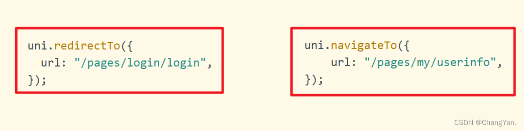
The difference between redirectto and navigateto in uniapp
Core knowledge of distributed cache
How engineers treat open source -- the heartfelt words of an old engineer

基于SSM框架的文章管理系统
48页数字政府智慧政务一网通办解决方案
Data analysis course notes (V) common statistical methods, data and spelling, index and composite index
What is a responsive object? How to create a responsive object?
DAY FOUR

【2022全网最细】接口测试一般怎么测?接口测试的流程和步骤
随机推荐
2021 SASE integration strategic roadmap (I)
Amazon MemoryDB for Redis 和 Amazon ElastiCache for Redis 的内存优化
2022/2/10 summary
TypeScript中使用类型别名
SQL的一种写法,匹配就更新,否则就是插入
Sword finger offer 26 Substructure of tree
MIT 6.824 - Raft学生指南
刘永鑫报告|微生物组数据分析与科学传播(晚7点半)
How rider uses nuget package offline
Leecode brushes questions and records interview questions 01.02 Determine whether it is character rearrangement for each other
Supersocket 1.6 creates a simple socket server with message length in the header
kubernetes部署ldap
DAY ONE
如何判断一个数组中的元素包含一个对象的所有属性值
The way of intelligent operation and maintenance application, bid farewell to the crisis of enterprise digital transformation
DAY FIVE
基于GO语言实现的X.509证书
DAY FOUR
DAY THREE
@TableId can‘t more than one in Class: “com.example.CloseContactSearcher.entity.Activity“.