[learning notes] numerical differentiation of back error propagation

The so-called numerical differentiation , In fact, to put it bluntly, it's derivative , Derivation includes direct derivation and partial derivation , What is used in neural networks is generally to find partial derivatives , Thus, the error of each weight is obtained .
Prepare to use this time Python To study a wave of numerical differentiation .

Direct derivation

Specific derivation formula , After learning advanced mathematics, you should know that there is a person named “ Forward differential ” Of course , His formula looks like this ：


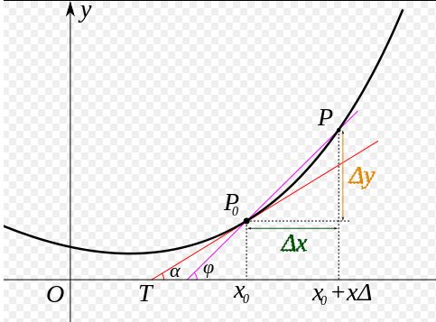
However, in Python In fact, it is not easy to realize , Because in this definition , The smaller the step of forward difference, the better , But in Pyhton The middle decimal point will not be kept so much . So when it is small to a certain extent, it becomes 0.
So in general “ Central difference ”, Namely x Add a step forward , Subtract one step backward , So it became ：

The result is the same as that above , Now we can use it Python Knock a wave of code implementation to see .

# Derivative function 
# Forward differential 
def forward_diff(f,x,h=1e-4):
    return (f(x+h)-f(x))/h
# Central difference 
def diff(f,x,h=1e-4):
    return (f(x+h)-f(x-h))/(2*h)
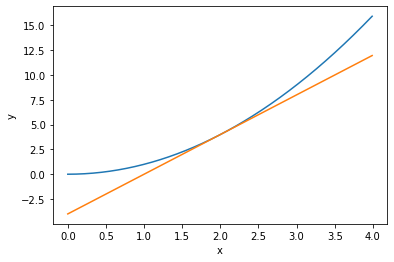
# Define a function ：y=x^2
def fun(x):
    return x**2
x = np.arange(0,4,0.01)
f = fun(x)
# Function in (2,4) Countdown at 
dy = diff(fun,2)
plt.plot(x,f)
# Use the formula of a straight line to draw the tangent 
plt.plot(x,dy*(x-2)+4)
plt.xlabel('x')
plt.ylabel('y')
plt.show()

Partial derivative and gradient

It's just an appetizer , The following is the main topic , That is to find partial derivatives of functions . This gradient is also a concept we came into contact with when learning how to calculate partial derivatives of functions .
If you still have an impression , We know that the partial derivative is a function , Let's say the following ：

There are two independent variables in this formula , So the derivation formula above is not easy to use . Because that formula only applies to the case of one independent variable . But it's not completely useless , That's it , When deriving from an independent variable , Just treat the other as a constant . This is what we did when we were studying advanced mathematics Finding partial derivatives . and gradient Is the vector formed by the partial derivative , The form of expression is as follows ：

So the gradient is a vector , He points to the lowest point of the function , That's the minimum . The above function has three variables , So there are three axes . Therefore, the displayed image is a three-dimensional image . So we can imagine , There is a concave piece on the ground , Then the gradient points to the lowest point of the concave .

After studying geography, you know the concept of contour , So the above graph changes into contour lines, which is how , The gradient is the lowest point pointing to the center . It's like playing with glass beads when we were young , Close to the middle hole , The glass bead will naturally slide to the lowest point of the hole .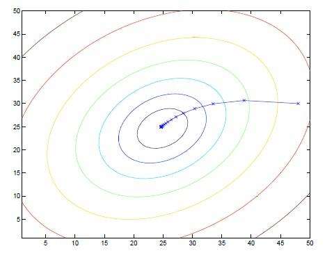

The old rules below , Or use it Python Look at the code .

def gradient(f,x,h=1e-4):
    # Gradient calculation 
    grad = np.zeros_like(x)
    for idx in range(x.size):
        tmp_val = x[idx]
        x[idx] = tmp_val + h
        fxh1 = f(x)
        x[idx] = tmp_val - h
        fxh2 = f(x)
        grad[idx] = (fxh1-fxh2)/(2*h)
        x[idx] = tmp_val
    return grad

Don't rush here , Let's learn another classic algorithm in machine learning , That is the gradient descent method , Then we'll see the effect .

Gradient descent method

Speaking of gradient descent method, this is classic , Although not the best algorithm , But it is the most practical , It's the easiest , His existence is to find a person called “ Global optimal solution ” Things that are . Nothing goes against my will , In fact, many times he will be trapped in “ Locally optimal solution ” The place of . Or we play with glass beads , When the glass bead rolls to the hole on the ground , As a result, there was a small hole on the way , So the glass beads can't be drawn in and out under the influence of gravity , In the end, it doesn't reach the hole you want .
This time is actually because no matter what the hole is , At the lowest end, the gradient is 0, When the gradient is 0 When , It is assumed by default that it is the place where the optimal solution is reached .
So the specific algorithm is actually very simple . First, we have an initialization coordinate , That is, the location of the original glass beads , Then we find the gradient value , Get a vector pointing to the lowest point of the ground . Then the glass beads can roll over （ This is definitely not a curse ）. But when you roll over , It's definitely impossible to roll over at one time , He has a “ step ”. It's like we walk , Going to the destination must be step by step , You can't fly directly , One step in place . So we also set up a system called “ Learning rate ” Things that are . Therefore, you can get the updated value of a calculation .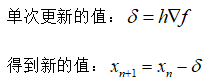

Here is the exciting code moment , We use it Python Draw a picture , And record the coordinates of each update , And show it .

# Minimum gradient function 
def grad_desc(f,init_x,lr=0.01,step=100):
    x = init_x
    x_history = []  # Record historical coordinate values 
    for i in range(step):
        x_history.append( x.copy() ) # Use numpy Of copy function , Not directly equal to 
        grad = gradient(f,x)
        x -= lr*grad
    return x,np.array(x_history)
# Define a function y=x1^2+x2^2
def fun1(x):
    return x[0]**2+x[1]**2
​
# Initialized coordinates 
init_x = np.array([-3.0,4.0])
lr = 0.1  # The default above is 0.01, Here you can reassign 
step = 20  # The default is 100, Reassign here 
x,x_history = grad_desc(fun1,init_x,lr=lr,step=step)
# Draw a coordinate 
plt.plot( [-5, 5], [0,0], '--b')
plt.plot( [0,0], [-5, 5], '--b')
# Draw updated scatter 
plt.plot(x_history[:,0], x_history[:,1], 'o')
# Limit the coordinate display range 
plt.xlim(-3.5, 3.5)
plt.ylim(-4.5, 4.5)
plt.xlabel("X1")
plt.ylabel("X2")
plt.show()

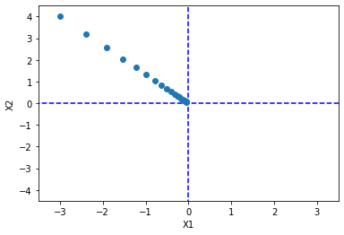
Pretty good , Effect grouping . It can be seen from the image , The farther the coordinate is from the minimum , The greater the gradient , Therefore, the larger the value of a single step update ; As it approaches the minimum , The gradient becomes smaller , So although the step size remains the same , But the value of a single update will also become smaller .
So how to determine the value of learning rate ？ The value of learning rate is 0 To 1 Between , It's too small , You can't even grow up . For example, we walk , Take big steps , There are also small ones . The big drawback is that it's easy to walk away at once , And it's easy to get stuck , Then I couldn't get to the smallest place . The learning rate is too small , Take too many steps , Very slow . So when the number of iterations is not enough , You haven't even reached your destination .
For example, I modify the learning rate to 0.05, Look at the results ：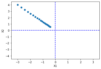

You can see , This iteration is over before it reaches the minimum , But you can just increase the number of iterations .
Then modify the learning rate to 0.3：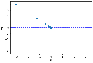

You can see , Take a big step ahead , All at once . The latter is due to the change of gradient value , So even if the learning rate is still very high , But I didn't cross my head . But what does not appear here does not mean that there will be no over crossing problem when the neural network algorithm is updated . Let's talk about this later .